Swarm conjunctions above the auroral oval
Contents
Swarm conjunctions above the auroral oval
Adrian Blagau (Institute for Space Sciences, Bucharest)
Joachim Vogt (Jacobs University Bremen)
Version Oct. 2020
This notebook accompanies the article “Multipoint Field-Aligned Current Estimates With Swarm” by A. Blagau, and J. Vogt, 2019. When used for publications, please acknowledge the authors’ work by citing the paper.
Introduction The different orbital velocities of Swarm upper and lower satellites makes possible a spacecraft alignment at certain orbital phase every other ~ 6.2 days. During such a time-interval, one can count several conjunction above the auroral oval (AO), depending on how strictly we require the satellite to line up. This notebook helps finding Swarm conjunctions above the AO, i.e. candidate events for the application of three-sat field-aligned current (FAC) density estimation method (see Vogt, Albert, and Marghitu, 2009).
The approach relies on an automatic procedure to identify the AO based on the unsigned FAC density in quasi-dipole coordinates interpreted as a normalized probability density function (pdf). Conjunctions are found by imposing temporal and spatial conditions (e.g. Swarm B and Swarm A/C to encounter an AO within a certain time-window, moving in the same hemisphere on the same upward/downward leg)
In the Input parameters section, the user could specify the time interval to search for conjunctions and the parameter that temporally constrains the conjunction. The spatial constraints are discussed in section Definition of s/c conjunction and could be changed by the user according to specific needs.
Since the automatic identification of AO location is not expected to work accurately in all cases, the list of events serves only for orientation. The standard plots generated at the end of the notebook are designed to help in (visually) assessing the quality of the conjunctions. Other requirements and critical aspects related to the application of three-sat method in the Swarm context (longitudinal separation, linear field variation, orientation of the spacecraft plane etc) are discussed in Blagau and Vogt, 2019.
Importing useful libraries (numpy, pandas, matplotlib, …)
# Uncomment if necessary:
# %matplotlib inline
# Uncomment for interactivity:
# %matplotlib widget

import numpy as np
import pandas as pd
from tqdm.auto import tqdm
from scipy import signal
from scipy.interpolate import interp1d
import datetime as dtm
import matplotlib.pyplot as plt
import matplotlib.dates as mdt

import warnings
warnings.filterwarnings('ignore')
Preparing to access ESA’s Swarm mission data and models from VirES environment
from viresclient import SwarmRequest
Defining some convenience functions
Computes the parameters of a low-pass Butterworth filter, if one decides to filter the data
fs = 1  # Sampling frequency
fc = 1./20.  # Cut-off frequency of a 20 s low-pass filter
w = fc / (fs / 2) # Normalize the frequency
butter_ord = 5
bf, af = signal.butter(butter_ord, w, 'low')
The function below splits a larger DataFrame in many smaller DataFrames, each corresponding to a certain time-interval. Used to split the Swarm data in half- or quarter-orbits.
def split_into_sections(df, begend_arr):
    """Splits the original dataframe df in sections according to
    time moments from begend_arr array. Returns a list of dataframes"""
    secorbs = []
    for start, end in zip(begend_arr[0:-1], begend_arr[1:]):
        secorb = df[start:end]
        secorbs.append(secorb)
    return secorbs
For an orbital section with monotonic variation in quasi-dipole latitude (QDLat), the function below finds the instance of time when the cumulative sum of unsigned FAC density (i.e. absolute value of current density) reaches its half maximum. This is returned as proxy for the FAC central time, together with other parameters like e.q. qd_trend (positive/ negative when QDLat is increasing/ decreasing), and qd_sign (indicates the upper/ lower hemisphere). The integration/ cumulative summing is performed as function of QDLat (not time), to correct for the non-linear changes in QDLat at the highest latitude.
def find_jabs_midcsum(df, fac_qnt = 'FAC_flt_sup', rez_qd = 100):
    """For a quarter-orbit section, finds the
    FAC central time, QDLat trend and QDLat sign"""
    qd = df['QDLat'].values
    qdlon = df['QDLon'].values
    jb = df[fac_qnt].values
    ti = df['QDLat'].index.values.astype(float)
    qd_trend = (qd[-1] - qd[0])/abs(qd[0] - qd[-1])  # >0 if QDLat inreases
    qd_sign = qd[0]/abs(qd[0])
    dqmin = np.round(np.amin(qd), decimals = 2)
    dqmax = np.round(np.amax(qd), decimals = 2)
    nr = round((dqmax - dqmin)*rez_qd + 1)
    qd_arr = np.linspace(dqmin, dqmax, nr)       # new QDLat array
    if qd_trend > 0:
        ti_arr = np.interp(qd_arr, qd, ti)          # time of new QD points
        jb_arr = np.interp(qd_arr, qd, jb)          # FAC at new QD points
    else:
        ti_arr = np.interp(qd_arr, qd[::-1], ti[::-1])
        jb_arr = np.interp(qd_arr, qd[::-1], jb[::-1])

    if np.sum(np.abs(jb_arr)) > 0:
        jabs_csum = np.cumsum(np.abs(jb_arr))/np.sum(np.abs(jb_arr))
        idx_jhalf = (np.abs(jabs_csum - 0.5)).argmin()
        idx_ti_ao = (np.abs(ti - ti_arr[idx_jhalf])).argmin()
        return ti_arr[idx_jhalf], qd_trend, qd_sign, qd_arr[idx_jhalf], \
                qdlon[idx_ti_ao], ti_arr, jb_arr, jabs_csum, qd_arr
    else:
        return np.nan, qd_trend, qd_sign, np.nan, \
                np.nan, ti_arr, jb_arr, np.nan, qd_arr
The function below is used only during the plotting part. Calls viresclient and provides magnetic field perturbation (in NEC or GEOC frame) for a specified time interval.
def get_db_data(sats, tbeg, tend, Bmodel, refframe = 'GEOC'):
    """Returns Swarm magnetic perturbation in a dataframe"""
    dti = pd.date_range(start = tbeg.round('s'),
                        end = tend.round('s'), freq='s', closed='left')
    ndti = len(dti)
    nsc = len(sats)
    Rsph = np.full((ndti,nsc,3),np.nan)
    dBnec = np.full((ndti,nsc,3),np.nan)
    dBgeo = np.full((ndti,nsc,3),np.nan)
    request = SwarmRequest()
    for sc in range(nsc):
        request.set_collection("SW_OPER_MAG"+sats[sc]+"_LR_1B")
        request.set_products(measurements=["B_NEC"],
                             models=[Bmodel],
                             residuals=True, sampling_step="PT1S")
        data = request.get_between(start_time = tbeg,
                                   end_time = tend,
                                   asynchronous=False, show_progress=False)
        print('Used MAG L1B file: ', data.sources[1])
        dat = data.as_dataframe()
        dsi = dat.reindex(index=dti, method='nearest')
        # store magnetic field perturbation in a data matrices
        dBnec[:,sc,:] = np.stack(dsi['B_NEC_res_CHAOS-all'].values, axis=0)
        coldBnec = pd.MultiIndex.from_product([['dBnec'],sats,['N','E','C']],
                                   names=['Var','Sat','Com'])
        dB = pd.DataFrame(dBnec.reshape(-1,nsc*3), columns=coldBnec,index=dti)
        if refframe == 'GEOC':
            Rsph[:,sc,:] = dsi[['Latitude','Longitude','Radius']].values
            latsc = np.deg2rad(Rsph[:,sc,0])
            lonsc = np.deg2rad(Rsph[:,sc,1])
            radsc = 0.001*Rsph[:,sc,2]
            # prepare conversion to global cartesian frame
            clt,slt = np.cos(latsc.flat),np.sin(latsc.flat)
            cln,sln = np.cos(lonsc.flat),np.sin(lonsc.flat)
            north = np.stack((-slt*cln,-slt*sln,clt),axis=-1)
            east = np.stack((-sln,cln,np.zeros(cln.shape)),axis=-1)
            center = np.stack((-clt*cln,-clt*sln,-slt),axis=-1)
            # read and convert magnetic field measurements
            bnecsc = dBnec[:,sc,:]
            dBgeo[:,sc,:] = np.matmul(np.stack((north,east,center),axis=-1),
                              bnecsc[...,None]).reshape(bnecsc.shape)
            coldBgeo = pd.MultiIndex.from_product([['dBgeo'],sats,['X','Y','Z']],
                                   names=['Var','Sat','Com'])
            dB = pd.DataFrame(dBgeo.reshape(-1,nsc*3), columns=coldBgeo,index=dti)
    return dB
Input parameters
Sets the time interval to search for Swarm conjunctions above the auroral oval. These occur in consecutive orbits every approx. 6 days. The magnetic field model(s) used to derive the magnetic field perturbation (shown in the standard plots) is also specified.
# Time range, satellites, and magnetic model
dtime_beg = '2014-05-04T15:00:00'
dtime_end = '2014-05-04T16:00:00'
twidth = 120
sats = ['A', 'B', 'C']
Bmodel="CHAOS-all='CHAOS-Core'+'CHAOS-Static'+'CHAOS-MMA-Primary'+'CHAOS-MMA-Secondary'"
Data retrieval and preparation
Uses viresclient to retrieve Swarm Level 2 single-sat. FAC data as well as auxiliary parameters, i.e. quasi-dipole latitude / longitude (QDLat / QDLon) and the magnetic local time (MLT) at spacecraft position.
For each satellite, the script downloads data corresponding to the full consecutive orbits that completely cover the original time-interval (i.e. a slightly larger interval is thus used) and stores it in the elements of dat_fac, which is a list of DataFrames objects. Note that:
In order to work with smaller arrays, only orbital sections where QDLat is \(> 45^{\,\circ}\) or \(<-45^{\,\circ}\) are retrieved.
The FAC data are also filtered using a low-pass Butterworth filter (column ‘FAC_flt’ in the DataFrame)
Since in the process of current integration, small FAC densities could badly affect the good identification of auroral oval, one possibility is to set to zero all current intensities below a certain value specified by the jthr parameter (column ‘FAC_flt_sup’ in the DataFrame)
%%time
jthr = 0.05  # threshold value for the FAC intensity
request = SwarmRequest()
nsc = len(sats)
orbs = np.full((nsc,2),np.nan)
dat_fac = []
tlarges = []
for sc in tqdm(range(nsc)):
    orb1 = request.get_orbit_number(sats[sc], dtime_beg, mission='Swarm')
    orb2 = request.get_orbit_number(sats[sc], dtime_end, mission='Swarm')
    print(orb1, orb2, orb2 - orb1)
    orbs[sc, :] = [orb1, orb2]
    large_beg, large_end = request.get_times_for_orbits(orb1, orb2, mission='Swarm', spacecraft=sats[sc])
    tlarges.append([large_beg, large_end])
    dti = pd.date_range(start = large_beg, end = large_end, freq='s', closed='left')
    # get FAC data for Northern hemisphere
    request.set_collection('SW_OPER_FAC'+sats[sc]+'TMS_2F')
    request.set_products(measurements=["FAC"],
                         auxiliaries=['QDLat','QDLon','MLT'],
                         sampling_step="PT1S")
    request.set_range_filter('QDLat', 45, 90)
    data = request.get_between(start_time = large_beg,
                               end_time = large_end,
                               asynchronous=True, show_progress=False)
    print('Used FAC file: ', data.sources[0])
    datN_fac = data.as_dataframe()
    request.clear_range_filter()
    # get FAC data for Southern hemisphere
    request.set_range_filter('QDLat', -90, -45)
    data = request.get_between(start_time = large_beg,
                               end_time = large_end,
                               asynchronous=True, show_progress=False)
    print('Used FAC file: ', data.sources[0])
    datS_fac= data.as_dataframe()
    request.clear_range_filter()
    # put toghether data from both hemispheres
    dat = pd.concat([datN_fac, datS_fac]).sort_index()
    dat['FAC_flt'] = signal.filtfilt(bf, af, dat['FAC'].values)
    dat['FAC_flt_sup'] = np.where(np.abs(dat['FAC_flt']) >= jthr, dat['FAC_flt'], 0)
    # append data from different satellites
    dat_fac.append(dat)
2492 2492 0
Used FAC file: SW_OPER_FACATMS_2F_20140504T000000_20140504T235959_0301
Used FAC file: SW_OPER_FACATMS_2F_20140504T000000_20140504T235959_0301
2480 2480 0
Used FAC file: SW_OPER_FACBTMS_2F_20140504T000000_20140504T235959_0301
Used FAC file: SW_OPER_FACBTMS_2F_20140504T000000_20140504T235959_0301
2488 2488 0
Used FAC file: SW_OPER_FACCTMS_2F_20140504T000000_20140504T235959_0301
Used FAC file:  SW_OPER_FACCTMS_2F_20140504T000000_20140504T235959_0301
CPU times: user 638 ms, sys: 143 ms, total: 780 ms
Wall time: 29.1 s
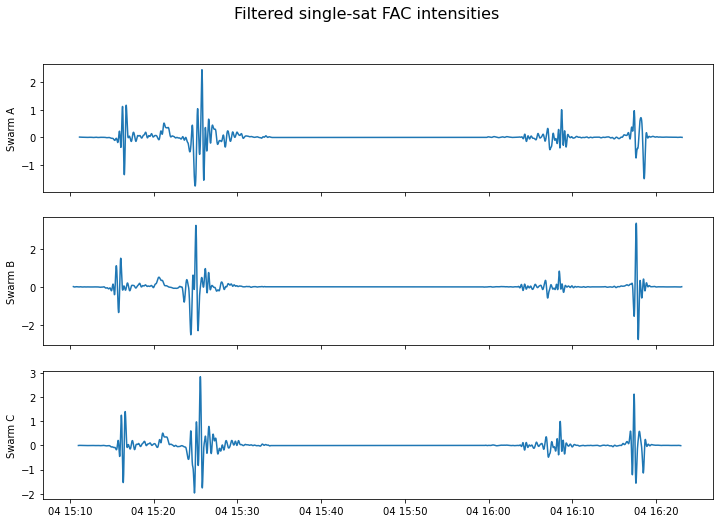
Plots the (filtered) L2 single-sat. FAC data over the whole interval
fig, (ax1, ax2, ax3) = plt.subplots(3, figsize=(12, 8), sharex='all')
fig.suptitle('Filtered single-sat FAC intensities', fontsize=16)
ax1.set_ylabel('Swarm A')
ax1.plot(dat_fac[0]['FAC_flt'])
ax2.set_ylabel('Swarm B')
ax2.plot(dat_fac[1]['FAC_flt'])
ax3.set_ylabel('Swarm C')
ax3.plot(dat_fac[2]['FAC_flt'])
[<matplotlib.lines.Line2D at 0x7fba2c6b8a60>]
Identification of auroral oval location
For each satellite, data is first split in half-orbit sections, corresponding to the Northern or Southern hemisphere. In the next stage, the half-orbit intervals are further split in quarter-orbits, using as separator the time instant when QDLat acquires its extreme value.
Then, for each quarter-orbit section, find_jabs_midcsum is called to estimate the central position of the auroral oval (approximated as the time when the cumulative sum of unsigned L2 FAC density reaches its half maximum). The function also returns the QDlat trend, sign, and value at central FAC for that quarter-orbit section.
After running the cell, the (three elements, i.e. one for each sat.) lists *_3sc contain np.arrays with FAC central times, QDlat trend, QDLat sign, QDLat value at central FAC, start and stop times for quarter-orbits when FAC intensity has value above the set threshold.
jabs_times_3sc, qd_trends_3sc, qd_signs_3sc, qd_aos_3sc, \
    qdlon_aos_3sc, beg_qor_3sc, end_qor_3sc = ([] for i in range(7))
for sc in range(nsc):
    # nr. of 1/2 orbits and 1/2 orbit duration
    nrho = int((orbs[sc,1] - orbs[sc,0] + 1)*2)
    dtho = (tlarges[sc][1] - tlarges[sc][0])/nrho
    # start and stop of 1/2 orbits
    begend_hor = [tlarges[sc][0] + ii*dtho for ii in range(nrho +1)]
    # splits DataFrame in 1/2 orbit sections; get time of maximum QDLat for each
    horbs = split_into_sections(dat_fac[sc], begend_hor)
    times_maxQDLat = [horbs[ii]['QDLat'].abs().idxmax().to_pydatetime() \
                    for ii in range(nrho)]
    begend_qor = sorted(times_maxQDLat + begend_hor)
    # splits DataFrame in 1/4 orbits sections;
    qorbs = split_into_sections(dat_fac[sc], begend_qor)
    # finds times when integrated absolute value of J reached its mid height
    jabs_times, qd_trends, qd_signs, qd_aos, qdlon_aos = \
        (np.full(len(qorbs),np.nan) for i in range(5))

    for jj in range(len(qorbs)):
        [jabs_times[jj], qd_trends[jj], qd_signs[jj], qd_aos[jj], \
         qdlon_aos[jj], ] = find_jabs_midcsum(qorbs[jj])[0:5]
    # keeps only 1/4 orbits when jabs_times is not np.nan (i.e with
    # points having current intensity above the set threshold)
    ind_notnan = np.flatnonzero(np.isfinite(jabs_times))
    jabs_times_3sc.append(jabs_times[ind_notnan])
    qd_trends_3sc.append(qd_trends[ind_notnan])
    qd_signs_3sc.append(qd_signs[ind_notnan])
    qd_aos_3sc.append(qd_aos[ind_notnan])
    qdlon_aos_3sc.append(qdlon_aos[ind_notnan])
    beg_qor_3sc.append(np.array(begend_qor)[ind_notnan])
    end_qor_3sc.append(np.array(begend_qor)[ind_notnan + 1])
Definition of s/c conjunction
To define Swarm near-conjunctions, one condition should involve the values of auroral central times, i.e. timesX (X=[A, B, C]). In addition, depending on the particular study, one needs to impose conditions on other quantities, like sign and trend of QDLat or QDLon values at central FAC.
For finding Swarm conjunctions at the beginning of the mission, when satellites revolve in the same direction along their orbits, one could use the conditions that timesX refer to the same branch of the orbit (same trend, i.e. ‘> 0’ in line 20 below. and sign of QDLat)
For finding conjunctions during the period of counter-rotating orbits, the above condition could change to impose different trends in QDLat for SwarmB and SwarmA/SwarmC, i.e. ‘< 0’ in line 20 below
For studies that look at FAC longitudinal gradients, one could require a separation in QDLon values at central FAC within a certain range (e.g. using the formula dLon = (QDLonA - QDLonB + 180) % 360 - 180 to compute longitudinal separation in degree).
The script below applies to the first situation listed above, using the following criteria:timesB within twidth limit from timesA or timesC
timesX refer to the same trend and sign of QDLat
After running the cell, conj_tbl (list of three elements, i.e. one for each sat.) contains the indexes of quarter-orbit intervals when Swarm satellites were in near-conjunction. Results are listed and stored in an ASCII file as: timesB , timesB - timesA, timesB - timesC, QDLat and QDLon values for each sat. at central FAC.
str_trange = dtime_beg.replace('-','')[:8]+'_'+ \
    dtime_beg.replace(':','')[11:15] + '_'+ \
    dtime_end.replace('-','')[:8] + '_'+ \
    dtime_end.replace(':','')[11:15]
fname_txt = 'swABC_conjunction_long_'+ str_trange + '.txt'
with open(fname_txt, 'w') as file:
        file.write('# time swB [%Y-%m-%dT%H:%M:%S], ' + \
                   'time diff. swA-swB, time diff. swC-swB,  ' + \
                   'QDLatA,  QDLatB,  QDLatC, QDLonA,  QDLonB,  QDLonC \n')
# moments when each s/c encounters the central auroral oval
timesA = pd.to_datetime(jabs_times_3sc[0])
timesB = pd.to_datetime(jabs_times_3sc[1])
timesC = pd.to_datetime(jabs_times_3sc[2])
conj_tbl = []
for indB in range(len(timesB)):
    indA = (np.abs(timesA - timesB[indB])).argmin()
    indC = (np.abs(timesC - timesB[indB])).argmin()
    if ((np.abs(timesA[indA] - timesB[indB]).total_seconds() <= twidth or \
        np.abs(timesC[indC] - timesB[indB]).total_seconds() <= twidth) and \
        (qd_trends_3sc[0][indA]*qd_trends_3sc[1][indB] > 0) and \
        (qd_signs_3sc[0][indA]*qd_signs_3sc[1][indB] > 0)):
        #(np.abs((qdlon_aos_3sc[1][indB] - qdlon_aos_3sc[0][indA] + \
        #         180) % 360 - 180) <= 40)):
        print(indB, timesB[indB].strftime('%Y-%m-%dT%H:%M:%S'), '  ',\
            str(int((timesA[indA] - timesB[indB]).total_seconds())), '  ',\
            str(int((timesC[indC] - timesB[indB]).total_seconds())), '  ', \
            str(round(qd_aos_3sc[0][indA],2)), '  ', \
            str(round(qd_aos_3sc[1][indB],2)), '  ', \
            str(round(qd_aos_3sc[2][indC],2)), '  ', \
            str(round(qdlon_aos_3sc[0][indA],2)), '  ', \
            str(round(qdlon_aos_3sc[1][indB],2)), '  ', \
            str(round(qdlon_aos_3sc[2][indC],2)))
        conj_tbl.append([indA, indB, indC])
        with open(fname_txt, 'a') as file:
            file.write(timesB[indB].strftime('%Y-%m-%dT%H:%M:%S') + '   ' +\
                str(int((timesA[indA] - timesB[indB]).total_seconds()))+ '   ' +\
                str(int((timesC[indC] - timesB[indB]).total_seconds()))+ '   ' +\
                str(round(qd_aos_3sc[0][indA],2))+ '   ' + \
                str(round(qd_aos_3sc[1][indB],2))+ '   ' + \
                str(round(qd_aos_3sc[2][indC],2))+ '   ' + \
                str(round(qdlon_aos_3sc[0][indA],2))+ '   ' + \
                str(round(qdlon_aos_3sc[1][indB],2))+ '   ' + \
                str(round(qdlon_aos_3sc[2][indC],2))+ '\n')
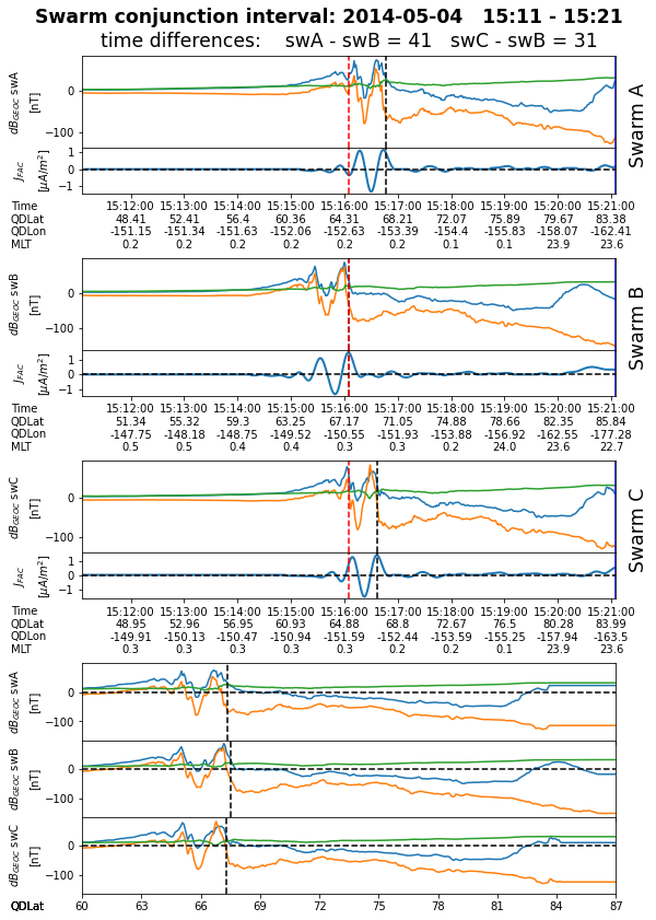
0 2014-05-04T15:16:05 41 31 67.33 67.51 67.31 -153.2 -150.66 -152.09
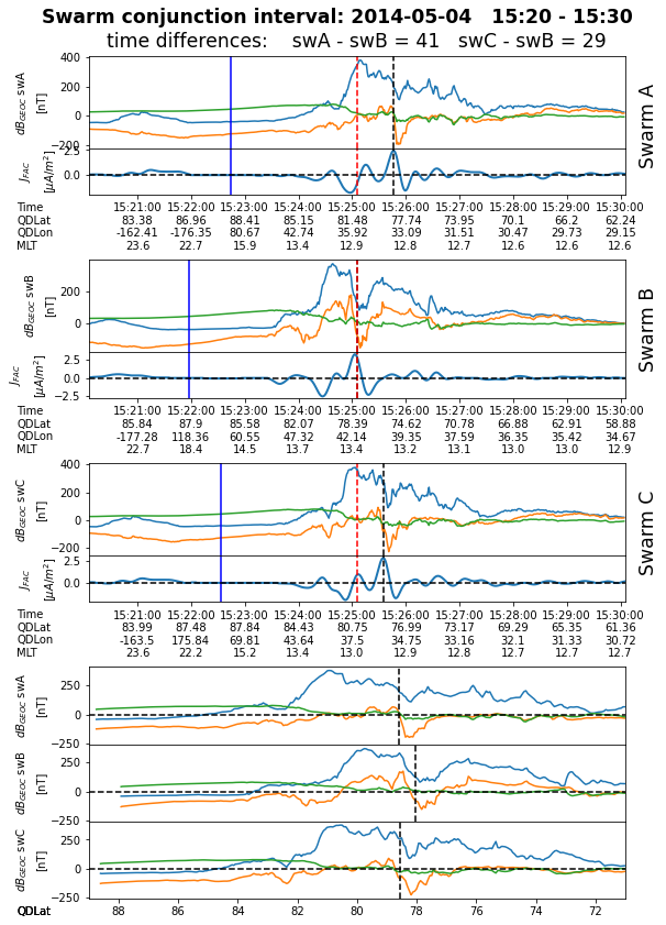
1 2014-05-04T15:25:05 41 29 78.58 78.05 78.54 33.58 41.81 35.67
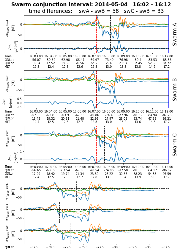
2 2014-05-04T16:07:09 58 33 -73.93 -71.39 -73.02 26.04 23.23 25.28
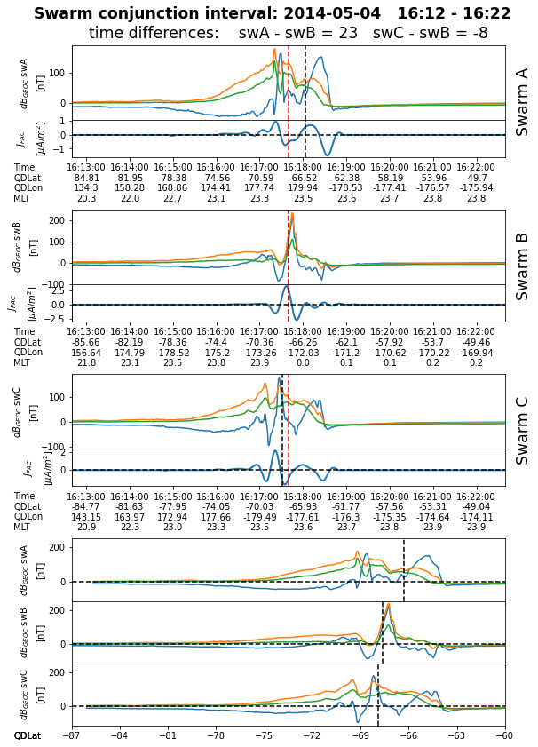
3 2014-05-04T16:17:39 23 -8 -66.31 -67.65 -67.9 -179.96 -172.4 -178.41
Plotting the results
Generates plots for the identified conjunctions, i.e. 10 minutes intervals centered on time instances listed above. The magnetic field perturbation in GEOC (obtained by calling get_db_data function) and (low-pass filtered) single-sat. FAC density data are plotted for each satellite. The auroral central times (i.e. Times[A,B,C]) and times when (unsigned) QDLat is maximum are indicated. The last three panels plot the magnetic field perturbation as a function of QDLat; QDLat values at central FAC is also indicated.
At the end, all the plots are collected in a multi-page pdf file.
fname_plots = 'plots_swABC_conjunction_long_'+ str_trange + '.pdf'

marg = pd.to_timedelta(300, unit='s')
list_plots = []
for kk in tqdm(range(len(conj_tbl))):
    print(kk)
    idxconj = conj_tbl[kk]
    dBgeo = get_db_data(sats, timesB[idxconj[1]] - marg, \
                        timesB[idxconj[1]] + marg, Bmodel)
    %run -i "plot_3sat_conjunction.py"
    list_plots.append(fname_fig)

list_plots_str = ' '.join(list_plots)
!gs -dNOPAUSE -sDEVICE=pdfwrite -sOUTPUTFILE={fname_plots} -dBATCH {list_plots_str}
0
Used MAG L1B file: SW_OPER_MAGA_LR_1B_20140504T000000_20140504T235959_0505_MDR_MAG_LR
Used MAG L1B file: SW_OPER_MAGB_LR_1B_20140504T000000_20140504T235959_0505_MDR_MAG_LR
Used MAG L1B file: SW_OPER_MAGC_LR_1B_20140504T000000_20140504T235959_0505_MDR_MAG_LR
1
Used MAG L1B file: SW_OPER_MAGA_LR_1B_20140504T000000_20140504T235959_0505_MDR_MAG_LR
Used MAG L1B file: SW_OPER_MAGB_LR_1B_20140504T000000_20140504T235959_0505_MDR_MAG_LR
Used MAG L1B file: SW_OPER_MAGC_LR_1B_20140504T000000_20140504T235959_0505_MDR_MAG_LR
2
Used MAG L1B file: SW_OPER_MAGA_LR_1B_20140504T000000_20140504T235959_0505_MDR_MAG_LR
Used MAG L1B file: SW_OPER_MAGB_LR_1B_20140504T000000_20140504T235959_0505_MDR_MAG_LR
Used MAG L1B file: SW_OPER_MAGC_LR_1B_20140504T000000_20140504T235959_0505_MDR_MAG_LR
3
Used MAG L1B file: SW_OPER_MAGA_LR_1B_20140504T000000_20140504T235959_0505_MDR_MAG_LR
Used MAG L1B file: SW_OPER_MAGB_LR_1B_20140504T000000_20140504T235959_0505_MDR_MAG_LR
Used MAG L1B file: SW_OPER_MAGC_LR_1B_20140504T000000_20140504T235959_0505_MDR_MAG_LR
GPL Ghostscript 9.50 (2019-10-15)
Copyright (C) 2019 Artifex Software, Inc.  All rights reserved.
This software is supplied under the GNU AGPLv3 and comes with NO WARRANTY:
see the file COPYING for details.
Processing pages 1 through 1.
Page 1
Processing pages 1 through 1.
Page 1
Processing pages 1 through 1.
Page 1
Processing pages 1 through 1.
Page 1