Three-sat FAC density estimation with Swarm
Contents
Three-sat FAC density estimation with Swarm
Adrian Blagau (Institute for Space Sciences, Bucharest)
Joachim Vogt (Jacobs University Bremen)
Version Feb. 2020
This notebook accompanies the article “Multipoint Field-Aligned Current Estimates With Swarm” by A. Blagau, and J. Vogt, 2019. When used for publications, please acknowledge the authors’ work by citing the paper.
Introduction The notebook makes use of the three-s/c gradient estimation method, developed in Vogt, Albert, and Marghitu, 2009 to estimates the field-aligned current (FAC) density from the Swarm measurements when the satellites are in a close configuration. A detailed discussion on applying the three-s/c method in the context of Swarm (notably selection of events and other critical aspects) is provided in Blagau and Vogt, 2019
In the Input parameters section, the user specifies the interval of analysis and the magnetic model(s) used to compute the magnetic field perturbation. Optionally, the sensor data can be shifted in time (tshift array) and/or can be filtered.
Importing useful libraries (numpy, pandas, matplotlib, …)
# Uncomment if necessary:
# %matplotlib inline
# Uncomment for interactivity:
# %matplotlib widget

import numpy as np
import pandas as pd
from tqdm.auto import tqdm
from scipy import signal
import matplotlib.pyplot as plt
import datetime as dtm
import matplotlib.dates as mdt

import warnings
warnings.filterwarnings('ignore')
Preparing to access ESA’s Swarm mission data and models from VirES environment
from viresclient import SwarmRequest
Defines some convenience functions
Computes the parameters of a low-pass Butterworth filter, if one decides to filter the data
fs = 1  # Sampling frequency
fc = 1./20.  # Cut-off frequency of a 20 s low-pass filter
w = fc / (fs / 2) # Normalize the frequency
butter_ord = 5
bf, af = signal.butter(butter_ord, w, 'low')
Defines recivec3s function to compute the reciprocal vectors for a three-s/c configuration
def recivec3s(R):
    Rc = np.mean(R, axis=-2)
    Rmeso = R - Rc[:, np.newaxis, :]
    r12 = Rmeso[:,1,:] - Rmeso[:,0,:]
    r13 = Rmeso[:,2,:] - Rmeso[:,0,:]
    r23 = Rmeso[:,2,:] - Rmeso[:,1,:]
    nuvec = np.cross(r12, r13)
    nuvec_norm = np.linalg.norm(nuvec, axis=-1, keepdims=True)
    nuvec = np.divide(nuvec, nuvec_norm)
    Q3S = np.stack((np.cross(nuvec,r23), np.cross(nuvec,-r13), np.cross(nuvec,r12)),axis = -2)
    Q3S = np.divide(Q3S, nuvec_norm[...,None])
    Qtens = np.sum(np.matmul(Q3S[:,:,:,None],Q3S[:,:,None, :]), axis = -3)
    Rtens = np.sum(np.matmul(Rmeso[:,:,:,None],Rmeso[:,:,None, :]), axis = -3)
    return Rc, Rmeso, nuvec, Q3S, Qtens, Rtens
Input parameters
Specifying the time interval, the satellites, the magnetic field model. Optionally, the sensor data can be shifted in time and/or can be filtered
dtime_beg = '2014-06-29T12:33:00'
dtime_end = '2014-06-29T12:38:00'
sats = ['A','B','C']
Bmodel="CHAOS-all='CHAOS-Core'+'CHAOS-Static'+'CHAOS-MMA-Primary'+'CHAOS-MMA-Secondary'"
#tshift = [0, 10, 4]  # optional time-shift introduced between the Swarm sensors
tshift = [0, 0, 0]
use_filter = False   # 'True' for filtering the data
Data retrieval and preparation
Reads from VirES the sat. position (Rsph), magnetic L1b measurement (Bsw), and magnetic field model (Bmod). The quality flag of VFM data, i.e. Flags_B in the L1b files, is read as well. For a description of Flags_B values see Swarm Level 1b Product Definition from the Swarm documentation. The script identifies (and leaves unchanged) poor quality data points, i.e. when Flags_B > 0, as well as data gaps (and fills them with the values of the nearest neighboring point).
dti = pd.date_range(start = dtime_beg, end = dtime_end, freq='s', closed='left')
ndti = len(dti)
nsc = len(sats)
datagaps={}
Rsph = np.full((ndti,nsc,3),np.nan)
Bsw = np.full((ndti,nsc,3),np.nan)
Bmod = np.full((ndti,nsc,3),np.nan)
FlagsB = np.full((ndti,nsc),np.nan)
request = SwarmRequest()
for sc in tqdm(range(nsc)):
    request.set_collection("SW_OPER_MAG"+sats[sc]+"_LR_1B")
    request.set_products(measurements=["B_NEC","Flags_B"],
                         models=[Bmodel],
                         sampling_step="PT1S")
    data = request.get_between(start_time = dtime_beg,
                               end_time = dtime_end,
                               asynchronous=False, show_progress=False)
    print('Used MAG L1B file: ', data.sources[1])
    dat = data.as_dataframe()
    datagaps[sats[sc]] = dti.difference(dat.index)
    dsi = dat.reindex(index=dti, method='nearest')
    # store position, magnetic field and magnetic model vectors in corresponding data matrices
    Rsph[:,sc,:] = dsi[['Latitude','Longitude','Radius']].values
    Bsw[:,sc,:] = np.stack(dsi['B_NEC'].values, axis=0)
    Bmod[:,sc,:] = np.stack(dsi['B_NEC_CHAOS-all'].values, axis=0)
    FlagsB[:,sc] = dsi['Flags_B'].values
# collect all data in a single DataFrame for inspection
colRsph = pd.MultiIndex.from_product([['Rsph'],sats,['Lat','Lon','Radius']],
                                   names=['Var','Sat','Com'])
dfRsph = pd.DataFrame(Rsph.reshape(-1,nsc*3),columns=colRsph,index=dti)

colBswBmod = pd.MultiIndex.from_product([['Bsw','Bmod'],sats,['N','E','C']],
                                   names=['Var','Sat','Com'])
dfBswBmod = pd.DataFrame(np.concatenate((Bsw.reshape(-1,nsc*3),
                                         Bmod.reshape(-1,nsc*3)),axis=1),
                         columns=colBswBmod,index=dti)

dfFB = pd.DataFrame(FlagsB.reshape(-1,nsc),columns=sats,index=dti)

RsphBswBmod = pd.merge(dfRsph, dfBswBmod, left_index=True, right_index=True)
Used MAG L1B file: SW_OPER_MAGA_LR_1B_20140629T000000_20140629T235959_0505_MDR_MAG_LR
Used MAG L1B file: SW_OPER_MAGB_LR_1B_20140629T000000_20140629T235959_0505_MDR_MAG_LR
Used MAG L1B file: SW_OPER_MAGC_LR_1B_20140629T000000_20140629T235959_0505_MDR_MAG_LR
Shows the first lines of data structure for inspection
RsphBswBmod.head()
| Var | Rsph | Bsw | Bmod | ||||||||||||||||||
|---|---|---|---|---|---|---|---|---|---|---|---|---|---|---|---|---|---|---|---|---|---|
| Sat | A | B | C | A | ... | C | A | B | C | ||||||||||||
| Com | Lat | Lon | Radius | Lat | Lon | Radius | Lat | Lon | Radius | N | ... | C | N | E | C | N | E | C | N | E | C |
| 2014-06-29 12:33:00 | -80.911390 | -65.774670 | 6851755.55 | -80.169390 | -61.467951 | 6900623.63 | -81.554000 | -63.031595 | 6851779.47 | 12732.0097 | ... | -37338.7848 | 12734.024209 | 6188.853291 | -37157.458968 | 12941.555713 | 5199.868902 | -35698.749635 | 12832.159674 | 5776.273701 | -37342.619704 |
| 2014-06-29 12:33:01 | -80.972259 | -65.660006 | 6851756.68 | -80.230700 | -61.386827 | 6900625.20 | -81.614416 | -62.898266 | 6851780.59 | 12728.3808 | ... | -37365.0720 | 12730.191872 | 6174.737562 | -37183.780781 | 12934.753470 | 5191.139742 | -35728.940568 | 12829.870849 | 5757.982971 | -37369.111138 |
| 2014-06-29 12:33:02 | -81.033090 | -65.543742 | 6851757.82 | -80.291988 | -61.304637 | 6900626.76 | -81.674782 | -62.762957 | 6851781.71 | 12724.2641 | ... | -37391.1771 | 12726.512653 | 6160.298355 | -37210.044344 | 12928.027208 | 5182.188523 | -35759.085743 | 12827.751426 | 5739.281490 | -37395.546731 |
| 2014-06-29 12:33:03 | -81.093880 | -65.425848 | 6851758.95 | -80.353253 | -61.221361 | 6900628.32 | -81.735100 | -62.625625 | 6851782.82 | 12720.9187 | ... | -37417.2302 | 12722.989087 | 6145.529018 | -37236.250076 | 12921.378343 | 5173.011078 | -35789.184950 | 12825.803900 | 5720.160144 | -37421.926831 |
| 2014-06-29 12:33:04 | -81.154631 | -65.306289 | 6851760.07 | -80.414497 | -61.136977 | 6900629.87 | -81.795367 | -62.486228 | 6851783.94 | 12717.7181 | ... | -37443.4390 | 12719.623649 | 6130.422607 | -37262.397986 | 12914.808375 | 5163.603280 | -35819.238413 | 12824.030626 | 5700.609473 | -37448.251130 |
5 rows × 27 columns
Prints a report about the quality of VFM data, i.e. the sum of Flags_B values for each satellite (ideally 0) and the number of missing data points (ideally 0). Print timestamps with nonzero Flags_B values or when data is missing (if applicable).
FBnonzero = dfFB.loc[ (dfFB.A > 0) | (dfFB.B > 0) | (dfFB.C > 0)]
FBnA = dfFB['A'].loc[ (dfFB.A > 0)]
FBnB = dfFB['B'].loc[ (dfFB.B > 0)]
FBnC = dfFB['C'].loc[ (dfFB.C > 0)]
print('Number of points with non-zero quality flag / missing data:')
print('Swarm A: ', FBnA.count(), ' / ', datagaps['A'].size)
print('Swarm B: ', FBnB.count(), ' / ', datagaps['B'].size)
print('Swarm C: ', FBnC.count(), ' / ', datagaps['C'].size)
print()
if dfFB.sum(axis=0).sum(0) :
    print('Time stamps with nonzero FlagsB:')
    print(FBnonzero)
if datagaps['A'].size :
    print('Missing data for Swarm A: ', datagaps['A'].values)
if datagaps['B'].size :
    print('Missing data for Swarm B: ', datagaps['B'].values)
if datagaps['C'].size :
    print('Missing data for Swarm C: ', datagaps['C'].values)
Number of points with non-zero quality flag / missing data:
Swarm A:  0  /  0
Swarm B:  0  /  0
Swarm C:  0  /  0
Computes sats positions (R), magnetic measurements (B), and magnetic field perturbations (dB) in the global geographic (Cartesian) frame. Takes care of the optional time-shifts introduced between the sensors. Filters the magnetic field perturbations if requested so.
ts = np.around(np.array(tshift) - min(tshift))
tsh3s = np.around(np.mean(ts), decimals=3)
ndt = ndti - max(ts)
dt = dti[:ndt].shift(1000.*tsh3s,freq='ms')  # new data timeline
R = np.full((ndt,nsc,3),np.nan)
B = np.full((ndt,nsc,3),np.nan)
dB = np.full((ndt,nsc,3),np.nan)
for sc in range(nsc):
    latsc = np.deg2rad(Rsph[ts[sc]:ts[sc]+ndt,sc,0])
    lonsc = np.deg2rad(Rsph[ts[sc]:ts[sc]+ndt,sc,1])
    radsc = 0.001*Rsph[ts[sc]:ts[sc]+ndt,sc,2]
    # prepare conversion to global cartesian frame
    clt,slt = np.cos(latsc.flat),np.sin(latsc.flat)
    cln,sln = np.cos(lonsc.flat),np.sin(lonsc.flat)
    north = np.stack((-slt*cln,-slt*sln,clt),axis=-1)
    east = np.stack((-sln,cln,np.zeros(cln.shape)),axis=-1)
    center = np.stack((-clt*cln,-clt*sln,-slt),axis=-1)
    # store cartesian position vectors in position data matrix R
    R[:,sc,:] = -radsc[...,None]*center
    # store magnetic field measurements in the same frame
    bnecsc = Bsw[ts[sc]:ts[sc]+ndt,sc,:]
    B[:,sc,:] = np.matmul(np.stack((north,east,center),axis=-1),
                              bnecsc[...,None]).reshape(bnecsc.shape)
    # store magnetic field perturbation in the same frame
    dbnecsc = Bsw[ts[sc]:ts[sc]+ndt,sc,:] - Bmod[ts[sc]:ts[sc]+ndt,sc,:]
    dB[:,sc,:] = np.matmul(np.stack((north,east,center),axis=-1),
                              dbnecsc[...,None]).reshape(dbnecsc.shape)
    if use_filter:
        dB[:,sc,:] = signal.filtfilt(bf, af, dB[:,sc,:], axis=0)
# collect all data in a single DataFrame
colRBdB = pd.MultiIndex.from_product([['R','B','dB'],sats,['x','y','z']],
                                   names=['Var','Sat','Com'])
RBdB = pd.DataFrame(np.concatenate((R.reshape(-1,nsc*3),B.reshape(-1,nsc*3),dB.reshape(-1,nsc*3)),axis=1),
                      columns=colRBdB,index=dt)
Reads two-s/s FAC estimate from the L2 product for later comparison
request.set_collection('SW_OPER_FAC_TMS_2F')
request.set_products(measurements="FAC", sampling_step="PT1S")
data = request.get_between(start_time = dtime_beg,
                               end_time = dtime_end,
                               asynchronous=False)
print('Used FAC file: ', data.sources[0])
FAC_L2 = data.as_dataframe()
Used FAC file: SW_OPER_FAC_TMS_2F_20140629T000000_20140629T235959_0301
Computes the FAC density and other parameters
Uses recivec3s() function to compute the mesocenter of the Swarm constellation (Rc), the s/c positions in the mesocentric frame (Rmeso), the direction normal to spacecraft plane (nuvec), the reciprocal vectors (Q3S), the reciprocal tensor (Qtens), and the position tensor (Rtens).
Rc, Rmeso, nuvec, Q3S, Qtens, Rtens = recivec3s(R)
Computes the direction of (un-subtracted) local magnetic field Bunit and the orientation of spacecraft plane with respect to Bunit (cosBN and angBN). Register (for later exclusion) data points where B vector is too close to the spacecraft plane, i.e. below a threshold value set in angTHR.
Bunit = B.mean(axis=-2)/np.linalg.norm(B.mean(axis=-2),axis=-1)[...,None]
cosBN = np.matmul(Bunit[...,None,:],nuvec[...,:,None]).reshape(dt.shape)
angBN = pd.Series(np.arccos(cosBN)*180./np.pi, index=dt)
angTHR = 25.
texcl = (np.absolute(angBN) < 90 + angTHR) & (np.absolute(angBN) > 90 - angTHR)
Estimates the curl of magnetic field perturbation curlB. Associates its normal / radial component curlBrad with an electric current of density Jfac, flowing along the magnetic field line.
muo = 4*np.pi*1e-7
CurlB = np.sum( np.cross(Q3S,dB,axis=-1), axis=-2 )
CurlBrad = np.matmul(CurlB[...,None,:],nuvec[...,:,None]).reshape(dt.shape)
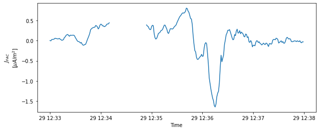
Jfac= (1e-6/muo)*pd.Series(CurlBrad/cosBN,index=dt)
Jfac.loc[texcl] = np.nan
plt.figure(figsize = [10,4])
plt.plot(Jfac)
plt.ylabel('$J_{FAC}$\n[$\mu A/m^2$]')
plt.xlabel('Time')
Text(0.5, 0, 'Time')
The condition number CN3 evaluates the stability of the solution (the quality of the Rtens inversion). The error errJ in FAC density due to (mutually uncorrelated and isotropic) instrumental noise is evaluated by considering a flat value db nT for δB
eigval = np.sort(np.linalg.eigvals(Rtens), axis=-1)
CN3 = pd.Series(np.log10(np.divide(eigval[:,2],eigval[:,1])),index=dt)

db = 0.5
if use_filter:
    db = 0.2
traceq = np.trace(Qtens, axis1=-2, axis2=-1)
errJ = 1e-6*db/muo*pd.Series(np.sqrt(traceq)/np.absolute(cosBN),index=dt)
errJ.loc[texcl] = np.nan
Plotting and saving the results
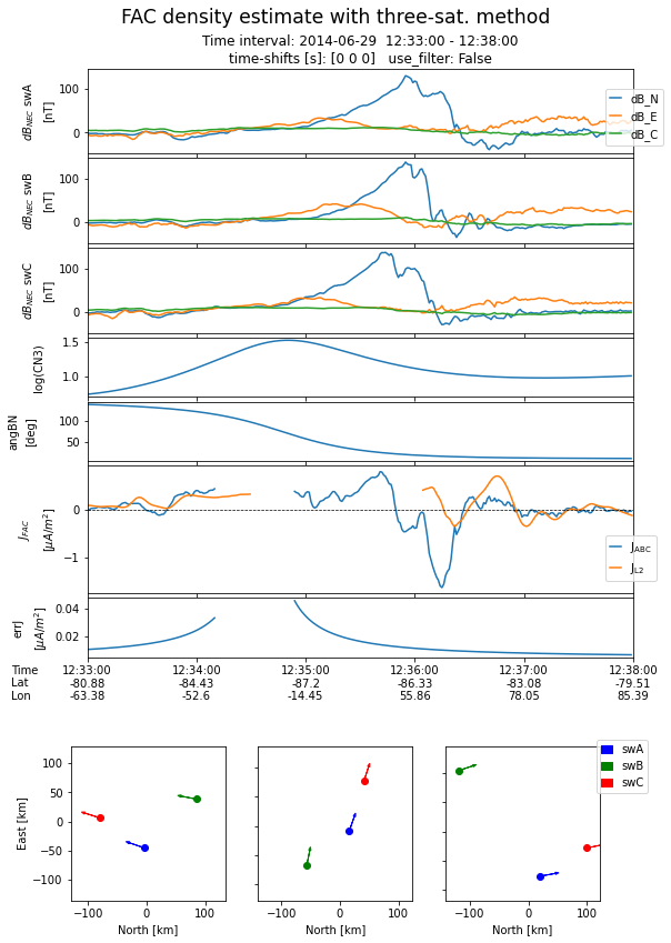
The script below produces a plot and two ASCII files, for the input data and for the results. A third ASCII file (input data quality report) is produced if non-zero quality flag and/or missing data points are present in the input data. The generated plot presents:
the NEC components of the magnetic field perturbation, dB, for all three satellites. A common range along y axes is used
the logarithm of the condition number, CN3
angle between the normal to the spacecraft plane and the direction of local ambient magnetic field.
comparison between the FAC density estimated with the three-s/c method and the ESA L2 FAC product obtained from the dual-s/c method.
the FAC estimation errors due to instrumental noise
The values for tick labels refer to the position of the mesocenter.
On the bottom, the spacecraft configurations are shown at three instances (i.e. beginning, middle, and end of the interval) projected on the NE plane of the local NEC coordinate frame tied to the mesocenter. The s/c velocity vectors are also indicated by arrows.
%run -i "plot_and_save_three_sat.py"