Swarm FAC quality indicators
Contents
Swarm FAC quality indicators
Adrian Blagau (Institute for Space Sciences, Bucharest)
Joachim Vogt (Jacobs University Bremen)
Version Dec. 2021
This notebook accompanies the article “Multipoint Field-Aligned Current Estimates With Swarm” by A. Blagau, and J. Vogt, 2019. When used for publications, please acknowledge the authors’ work by citing the paper.
Introduction A set of quality indicators is calculated for each auroral oval (AO) crossing within the specified interval. After an automatic identification of AO location, the MVA technique and the correlation analysis are used to characterize the FAC sheet planarity, inclination and stationarity. Being closely related to the underlying assumptions used in different FAC density estimation technique, the indicators are meant to help the users in assessing the quality of these estimations.
To easily follow the logical flow in the notebook, the functions listed below are put in the accompanying funcs_quality_indicators.py python script:
split_into_sections : splits a DataFrame in a list of DataFrames
normvec : computes the unit-vectors of a vector time series
rotvecax : rotates a vector by an angle around another vector
sign_ang : returns the signed angle between two vectors
R_B_dB_in_GEOC : transforms in GEO Cartesian frame the satellite position (initially in spherical coordinates) and magnetic field & perturbation (initially in NEC)
singleJfac : computes the single-satellite FAC density
find_ao_margins : estimates the margins of auroral oval on a quarter-orbit interval
mva : performs MVA and constrained MVA on an array of 3D vector
In the Input parameters section, the user could specify the time interval to search for conjunctions and the parameter that temporally constrains the conjunction. The spatial constraints are discussed in section Definition of s/c conjunction and could be changed by the user according to specific needs.
Importing useful libraries (numpy, pandas, matplotlib, …)
# Uncomment if necessary:
# %matplotlib inline
# Uncomment for interactivity:
# %matplotlib widget

import numpy as np
import pandas as pd
from scipy import signal
from scipy.interpolate import interp1d
import datetime as dtm
from datetime import timezone
import matplotlib.pyplot as plt
import matplotlib.dates as mdt

from funcs_fac import *

import warnings
warnings.filterwarnings('ignore')
Prepare to access ESA’s Swarm mission data and models from VirES environment
from viresclient import SwarmRequest
Defining some convenience functions
Computes the parameters of a low-pass Butterworth filter, if one decides to filter the data
fs = 1  # Sampling frequency
fc = 1./20.  # Cut-off frequency of a 20 s low-pass filter
w = fc / (fs / 2) # Normalize the frequency
butter_ord = 5
bf, af = signal.butter(butter_ord, w, 'low')
Function to perform the MVA on an array of 3D vectors. To do the analysis in a plane (e.g. perpendicular to the local average magnetic field), the normal to that plane cdir (3D vector) should be specified.
def mva(v, cdir = None):
    # returns results of MVA on the array of 3D vector v. If cdir (3D vector)
    # is provided, the analysis is performed in the plane perpendiculat to it
    v_cov = np.cov(v, rowvar=False, bias=True)
    if cdir is not None:
        ccol = cdir.reshape(3,1)
        cunit = ccol / np.linalg.norm(ccol)
        d_mat = (np.identity(3) - np.dot(cunit,cunit.T))
        v_cov = np.matmul(np.matmul(d_mat, v_cov), d_mat)
    return np.linalg.eigh(v_cov)
Input parameters
Sets the time interval for analysis and the satellite pair, typically Swarm A and C. The magnetic field model(s) used to derive the magnetic field perturbation (shown in the standard plots) is also specified.
# Time range, satellites, and magnetic model
dtime_beg = '2014-05-04T04:00:00'
dtime_end = '2014-05-04T04:00:00'

sats = ['A', 'C']
Bmodel="CHAOS-all='CHAOS-Core'+'CHAOS-Static'+'CHAOS-MMA-Primary'+'CHAOS-MMA-Secondary'"
Data retrieval and preparation
Uses viresclient to retrieve Swarm Level 1b data as well as the (auxiliary parameter) quasi-dipole latitude. In order to work with smaller arrays, only orbital sections where |QDLat| is \(> 45^{\,\circ}\) are retrieved.
For each satellite, the script downloads data corresponding to the full consecutive orbits that completely cover the original time-interval (i.e. a slightly larger interval is thus used). Spacecraft position, magnetic field, and magnetic field perturbation are stored in dat_Bnec, which is a DataFrame structure.
%%time
request = SwarmRequest()
nsc = len(sats)
orbs = np.full((nsc,2),np.nan)
dat_Bnec = []
tlarges = []
for sc in range(nsc):
    orb1 = request.get_orbit_number(sats[sc], dtime_beg, mission='Swarm')
    orb2 = request.get_orbit_number(sats[sc], dtime_end, mission='Swarm')
    print(orb1, orb2, orb2 - orb1)
    orbs[sc, :] = [orb1, orb2]
    large_beg, large_end = request.get_times_for_orbits(orb1, orb2, mission='Swarm', spacecraft=sats[sc])
    tlarges.append([large_beg, large_end])
    dti = pd.date_range(start = large_beg, end = large_end, freq='s', closed='left')
    # get B NEC data for Northern hemisphere
    request.set_collection("SW_OPER_MAG"+sats[sc]+"_LR_1B")
    request.set_products(measurements=["B_NEC"],
                         auxiliaries=['QDLat','QDLon','MLT'],
                         models=[Bmodel],
                         sampling_step="PT1S")
    request.set_range_filter('QDLat', 45, 90)
    data = request.get_between(start_time = large_beg,
                               end_time = large_end,
                               asynchronous=True)
    print('Used MAG L1B file: ', data.sources[1])
    datN_Bnec = data.as_dataframe()
    request.clear_range_filter()
    # get B NEC data for Southern hemisphere
    request.set_range_filter('QDLat', -90, -45)
    data = request.get_between(start_time = large_beg,
                               end_time = large_end,
                               asynchronous=True)
    print('Used MAG L1B file: ', data.sources[1])
    datS_Bnec= data.as_dataframe()
    request.clear_range_filter()
    # put toghether data from both hemispheres
    dat = pd.concat([datN_Bnec, datS_Bnec]).sort_index()
    dat['dB_NEC'] = dat['B_NEC'].values - dat['B_NEC_CHAOS-all'].values
    # append data from different satellites
    dat_Bnec.append(dat)
2485 2485 0
Used MAG L1B file: SW_OPER_MAGA_LR_1B_20140504T000000_20140504T235959_0505_MDR_MAG_LR
Used MAG L1B file: SW_OPER_MAGA_LR_1B_20140504T000000_20140504T235959_0505_MDR_MAG_LR
2481 2481 0
Used MAG L1B file: SW_OPER_MAGC_LR_1B_20140504T000000_20140504T235959_0505_MDR_MAG_LR
Used MAG L1B file:  SW_OPER_MAGC_LR_1B_20140504T000000_20140504T235959_0505_MDR_MAG_LR
CPU times: user 681 ms, sys: 133 ms, total: 813 ms
Wall time: 24.4 s
Splitting the data in quarter orbit sections
For each satellite, data is first split in half-orbit sections, corresponding to the Northern or Southern hemisphere. In the next stage, the half-orbit intervals are further split in quarter-orbits, using as separator the time instant when QDLat acquires its extreme value. qorbs_Bnec is a list of DataFrame structures, each covering one quarter-orbit interval.
qorbs_Bnec = [[],[]]
for sc in range(nsc):
    # nr. of 1/2 orbits and 1/2 orbit duration
    nrho = int((orbs[sc,1] - orbs[sc,0] + 1)*2)
    dtho = (tlarges[sc][1] - tlarges[sc][0])/nrho
    # start and stop of 1/2 orbits
    begend_hor = [tlarges[sc][0] + ii*dtho for ii in range(nrho +1)]
    # split DataFrame in 1/2 orbit sections; get time of maximum QDLat for each
    horbs = split_into_sections(dat_Bnec[sc], begend_hor)
    times_maxQDLat = [horbs[ii]['QDLat'].abs().idxmax().to_pydatetime() \
                    for ii in range(nrho)]
    begend_qor = sorted(times_maxQDLat + begend_hor)
    # split DataFrame in 1/4 orbit sections;
    qorbs_Bnec[sc] = split_into_sections(dat_Bnec[sc], begend_qor)

nrq = len(qorbs_Bnec[0]) # total nr. of 1/4 orbits
FAC density and magnetic perturbation in GEO frame
For each quarter-orbit, transforms the magnetic field in GEO frame and computes the FAC density by applying the single-satellite method on the filtered magnetic data. qorbs_dB and qorbs_fac are list of DataFrame structures containing the corresponding data
qorbs_dB = [[],[]]
qorbs_fac = [[],[]]
jthr = 0.05  # threshold value for the FAC intensity
for sc in range(nsc):
    for jj in range(nrq):
        # store position, magnetic field and magnetic model vectors as data array
        Rsph = qorbs_Bnec[sc][jj][['Latitude','Longitude','Radius']].values
        Bnec = np.stack(qorbs_Bnec[sc][jj]['B_NEC'].values, axis=0)
        Bmod = np.stack(qorbs_Bnec[sc][jj]['B_NEC_CHAOS-all'].values, axis=0)
        dBnec = np.stack(qorbs_Bnec[sc][jj]['dB_NEC'].values, axis=0)
        ti = qorbs_Bnec[sc][jj].index
        R, B, dB = R_B_dB_in_GEOC(Rsph, Bnec, dBnec)
        dB_flt = signal.filtfilt(bf, af, dB, axis=0)
        colBdB = pd.MultiIndex.from_product([['Rgeo','Bgeo','dBgeo','dBgeo_flt','dBnec'],\
                                    ['x','y','z']], names=['Var','Com'])
        qorbs_dB[sc].append(pd.DataFrame(np.concatenate((R.reshape(-1,3), B.reshape(-1,3), \
                        dB.reshape(-1,3), dB_flt.reshape(-1,3),\
                        dBnec.reshape(-1,3)),axis=1), columns=colBdB,index=ti))
        tt, Rmid, jb_flt,_,_,_,_,_ = singleJfac(ti, R, B, dB_flt)
        QDlat_ti = qorbs_Bnec[sc][jj]['QDLat'].values
        tt64 = tt.astype("int64")
        ti64 = ti.asi8
        QDLat_tt = np.interp(tt64, ti64, QDlat_ti)
        jb_flt_sup = np.where(np.abs(jb_flt) >= jthr, jb_flt, 0)
        qorbs_fac[sc].append(pd.DataFrame(np.concatenate((QDLat_tt[:,np.newaxis], \
                        jb_flt[:,np.newaxis], jb_flt_sup[:,np.newaxis]),axis = 1),\
                         columns=['QDLat','FAC_flt','FAC_flt_sup'], index=tt))
Estimation of AO margins
For each quarter-orbit section, find_ao_margins is called to automatically estimate the margins of the auroral oval. For that purpose:
the FAC data based on (low-pass Butterworth) filtered magnetic field perturbation are considered
the cumulative sum (integral) of unsigned FAC density is computed. The integration is performed as function of QDLat (not time), to correct for the non-linear changes in QDLat at the highest latitude.
since in the process of current integration, small FAC densities could badly affect the good identification of auroral oval, only current densities above a certain value, specified by the jthr parameter, is considered
the first, i.e. Q1, and the third, i.e. Q3, quartiles are computed. and the AO margins are estimated as Q1 - (O3-Q1) and Q3 + (O3-Q1)
tbeg_ao, tcen_ao, tend_ao, tbeg_mva, tend_mva = \
            (np.full((nsc,nrq),pd.NaT) for i in range(5))
for sc in range(nsc):
    for jj in range(nrq):
        tbeg_ao[sc][jj], tcen_ao[sc][jj], tend_ao[sc][jj] = \
            find_ao_margins(qorbs_fac[sc][jj])[0:3]
        tbeg_mva[sc][jj] = tbeg_ao[sc][jj].ceil(freq = 's')
        tend_mva[sc][jj] = tend_ao[sc][jj].floor(freq = 's')
MVA analysis
For each quarter-orbit section, MVA in performed on the AO interval in the plane perpendicular to the average magnetic field direction. The current sheet normal is provided by the eigenvector associated with the minimum magnetic variance, while the sense of direction is chosen according to the sat. velocity
qorbs_mva = [[],[]]
lbd_min, lbd_max, ang_vn = (np.full((nsc,nrq),np.nan) for i in range(3))
dir_bunit, dir_min, dir_max= (np.full((nsc,nrq,3),np.nan) for i in range(3))
for sc in range(nsc):
    for jj in range(nrq):
        ti_un = qorbs_dB[sc][jj].index.values
        dB_un = qorbs_dB[sc][jj]['dBgeo'].values
        B_un = qorbs_dB[sc][jj]['Bgeo'].values
        R_un = qorbs_dB[sc][jj]['Rgeo'].values
        # eV2d is the satellite velocity in the tangent plane
        # (i.e. perpendicular to position vector)
        V3d = R_un[1:,:] - R_un[:-1,:]
        Rmid = 0.5*(R_un[1:,:] + R_un[:-1,:])
        eV3d, eRmid = normvec(V3d), normvec(Rmid)
        eV2d = normvec(np.cross(eRmid, np.cross(eV3d, eRmid)))
        # select quantities for MVA interval and remove NaN points
        indok = np.where((ti_un >= tbeg_mva[sc][jj]) & \
                         (ti_un <= tend_mva[sc][jj]) & \
                         ~np.isnan(dB_un[:,0]))[0]
        dB_int, B_int = dB_un[indok,:], B_un[indok,:]
        B_ave = np.average(B_int, axis = 0)
        B_unit = B_ave / np.linalg.norm(B_ave)
        # apply constrained MVA
        eigval,eigvec = mva(dB_int, cdir=B_unit)
        # select the minvar orientation according to sat. velocity
        eV3d_ave = np.average(eV3d[indok[:-1]], axis = 0)
        mindir = eigvec[:,1]
        if np.sum(mindir*eV3d_ave) < 0:
            mindir = -eigvec[:,1]
        maxdir = np.cross(B_unit, mindir)
        lbd_min[sc, jj], lbd_max[sc, jj] = eigval[1], eigval[2]
        dir_bunit[sc,jj,:] = B_unit
        dir_min[sc,jj,:] = mindir
        dir_max[sc,jj,:] = maxdir

        # compute the FAC inclination wrt sat. velocity in the tangential plane
        eN2d, ang = eV2d.copy(), np.zeros(len(ti_un))
        eN2d[indok[:-1]] = \
            normvec(np.cross(eRmid[indok[:-1]], np.cross(mindir, eRmid[indok[:-1]])))

        cross_v_n = np.cross(eV2d[indok[:-1]], eN2d[indok[:-1]])
        sign_ang = np.sign(np.sum(eRmid[indok[:-1]]*cross_v_n, axis=-1))
        ang[indok[:-1]]  = \
            np.degrees(np.arcsin(sign_ang*np.linalg.norm(cross_v_n, axis=-1)))
        ang[0:indok[0]] = ang[indok[0]]
        ang[indok[-1]:] = ang[indok[-2]]
        ang_vn[sc][jj] = np.round(np.mean(ang[indok[:-1]]), 1)

        # transform magnetic perturbation in MVA frame
        geo2mva = np.stack((B_unit, mindir, maxdir), axis=1)
        dB_mva = np.matmul(qorbs_dB[sc][jj]['dBgeo'].values, geo2mva)
        qorbs_mva[sc].append(\
            pd.DataFrame(np.concatenate((dB_mva, ang[:,np.newaxis]),axis = 1),\
            columns=(['dB_B', 'dB_min', 'dB_max', 'ang_v_n']), index=ti_un))

        print('sw'+sats[sc]+' MVA interval: ', \
                  tbeg_mva[sc][jj], '  ', tend_mva[sc][jj])
        print('B_unit= %10.2f'%eigval[0], np.round(B_unit, decimals=4))
        print('mindir= %10.2f'%eigval[1], np.round(mindir, decimals=4))
        print('maxdir= %10.2f'%eigval[2], np.round(maxdir, decimals=4))
        print('')
swA MVA interval:  2014-05-04 04:12:09    2014-05-04 04:18:45
B_unit=      -0.00 [-0.4425  0.5314 -0.7224]
mindir=    5793.98 [-0.6405  0.3766  0.6693]
maxdir=    9861.21 [0.6277 0.7588 0.1737]

swA MVA interval:  2014-05-04 04:25:03    2014-05-04 04:27:52
B_unit=       0.00 [ 0.0445 -0.2575 -0.9652]
mindir=     923.45 [-0.334   0.9068 -0.2573]
maxdir=   52204.95 [ 0.9415  0.3339 -0.0457]

swA MVA interval:  2014-05-04 05:01:31    2014-05-04 05:02:40
B_unit=       0.00 [-0.094   0.5799 -0.8092]
mindir=    2426.93 [ 0.1768 -0.7902 -0.5868]
maxdir=   79799.41 [-0.9797 -0.1982 -0.0283]

swA MVA interval:  2014-05-04 05:10:19    2014-05-04 05:16:05
B_unit=       0.00 [ 0.228  -0.4169 -0.8799]
mindir=     635.15 [ 0.1561 -0.8764  0.4557]
maxdir=   30816.17 [-0.9611 -0.2413 -0.1347]

swC MVA interval:  2014-05-04 04:12:19    2014-05-04 04:18:46
B_unit=      -0.00 [-0.4479  0.5066 -0.7367]
mindir=    6994.60 [-0.891  -0.185   0.4146]
maxdir=    9327.77 [0.0737 0.8421 0.5342]

swC MVA interval:  2014-05-04 04:24:50    2014-05-04 04:27:49
B_unit=      -0.00 [ 0.0527 -0.2571 -0.965 ]
mindir=    1359.43 [-0.3166  0.9122 -0.2603]
maxdir=   51050.64 [ 0.9471  0.3192 -0.0333]

swC MVA interval:  2014-05-04 05:01:12    2014-05-04 05:02:36
B_unit=       0.00 [-0.1174  0.5782 -0.8074]
mindir=    2401.55 [ 0.1391 -0.7954 -0.5899]
maxdir=   67210.88 [-0.9833 -0.1816  0.0129]

swC MVA interval:  2014-05-04 05:10:25    2014-05-04 05:15:23
B_unit=      -0.00 [ 0.232  -0.4048 -0.8845]
mindir=     915.83 [ 0.1537 -0.8826  0.4443]
maxdir=   34185.63 [-0.9605 -0.239  -0.1426]
Correlation analysis
For each quarter-orbit section, the correlation of magnetic perturbations (correlation coefficient at optimum time lag) is computed. For that purpose:
for each satellite, the magnetic field perturbations along the maximum variance direction is used
satellite with narrower MVA interval is taken as reference. The running mean square deviation between magnetic perturbations within the reference interval and intervals from the second satellite up to 30 sec. ahead or below is computed
the correlation coefficient at optimum time lag (time lag that minimizes the mean square deviation) is computed
dt_mva = tend_mva - tbeg_mva
qorbs_ref_cc = []
opt_lag_ls, iref_arr = (np.full(nrq,np.nan, dtype='int') for i in range(2))
cc_ls = np.full(nrq,np.nan)
for jj in range(nrq):
    # set the reference s/c (i.e. the one with smaller MVA interval)
    iref = np.argmin(dt_mva[:,jj])
    isec = (iref +1) % 2
    iref_arr[jj] = iref
    sc_ref = sats[iref]
    sc_sec = sats[isec]

    # quarter orbit time and data for the second and reference s/c
    tsec = qorbs_mva[isec][jj].index
    dBsec = qorbs_mva[isec][jj]['dB_max'].values

    tref = qorbs_mva[iref][jj].index
    dBref = qorbs_mva[iref][jj]['dB_max'].values

    # index and data of MVA interval for reference s/c
    imva = np.where((tref >= tbeg_mva[iref][jj]) & \
                    (tref <= tend_mva[iref][jj]))
    dBref_mva = qorbs_mva[iref][jj]['dB_max'].values[imva]

    # set reference moment & index (here start of MVA inf for ref. s/c)
    ref_mom = tbeg_mva[iref][jj]
    ind_beg_tsec = np.where((tsec == ref_mom))[0][0]

    # nr. of points in MVA int
    nmva = int(dt_mva[iref,jj].total_seconds() + 1)

    # choose time-lags between -/+ 30 sec but takes care whether this is possible
    imin = int(np.max([-30, (np.min(tsec) - tbeg_mva[iref,jj]).total_seconds()]))
    imax = int(np.min([30, (np.max(tsec) - tend_mva[iref,jj]).total_seconds()]))
    nlags = int(imax - imin +1)  # nr. of time lags

    ls_run = np.full((nlags), np.nan)
    for ii in range(imin, imax+1):
        dBsec_run = dBsec[ind_beg_tsec+ii: ind_beg_tsec+ii+nmva]
        ls_run[ii-imin] = np.linalg.norm(dBsec_run - dBref_mva)/len(dBref_mva)

    best_ind_ls = np.argmin(ls_run)
    opt_lag_ls[jj] = best_ind_ls + imin

    dBsec_opt = dBsec[ind_beg_tsec+opt_lag_ls[jj] : ind_beg_tsec+opt_lag_ls[jj] + nmva]
    cc_ls[jj] = np.corrcoef(dBsec_opt, dBref_mva)[0,1]

    qorbs_ref_cc.append(pd.DataFrame(dBref_mva,index=\
        tsec[ind_beg_tsec+best_ind_ls+imin:ind_beg_tsec+best_ind_ls+imin + nmva]))
Saving the results
The results from MVA and correlation analysis, detailed for each quarter-orbit section, are saved locally in an ASCII file.
tlarge_beg = min([tlarges[0][0],tlarges[1][0]])
tlarge_end = max([tlarges[0][1],tlarges[1][1]])
str_fname = tlarge_beg.strftime("%Y%m%d_%H%M%S") +\
           '_' + tlarge_end.strftime("%Y%m%d_%H%M%S")

fname_out = 'QI_sw'+sats[0] + sats[1]+'_'+ str_fname +'.dat'

with open(fname_out, 'w') as file:
    file.write('Quality indices for satellites:  sw'+sats[0]+', sw'+sats[1]+'\n')
    file.write('Time interval: '+ tlarge_beg.strftime("%Y%m%d_%H%M%S") +\
               '  ' + tlarge_end.strftime("%Y%m%d_%H%M%S")+ '\n\n')

for jj in range(nrq):
    %run -i "save_qi.py"

file.close()
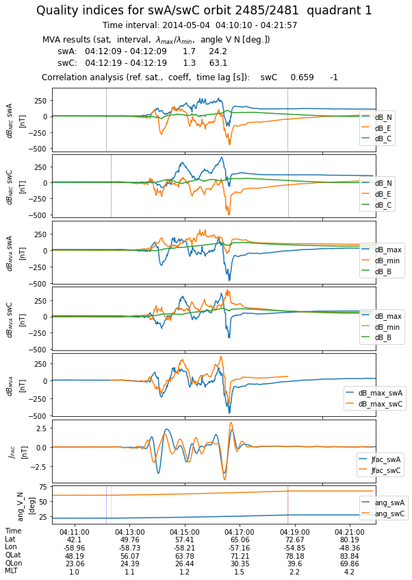
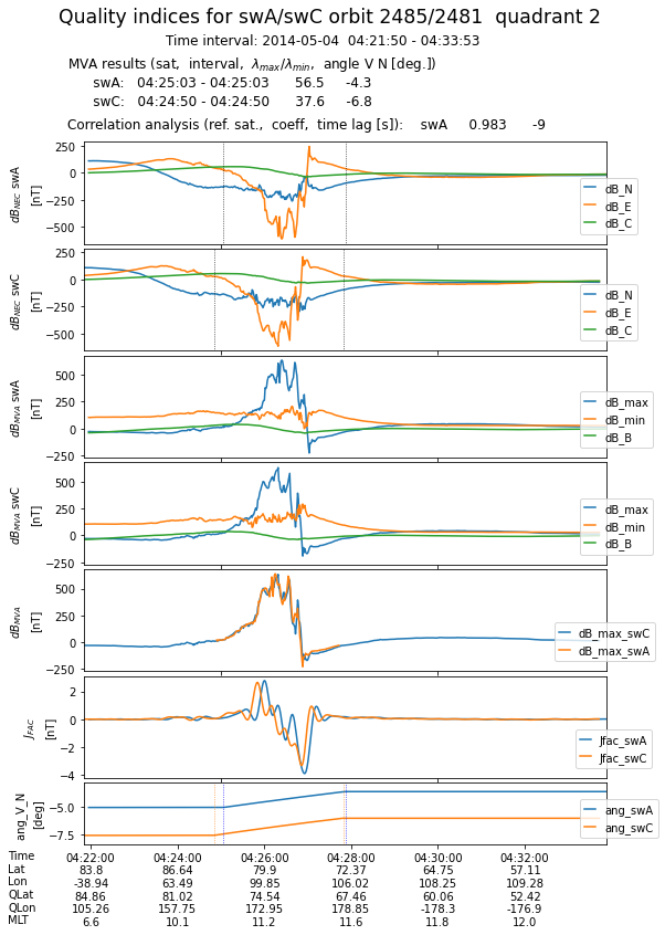
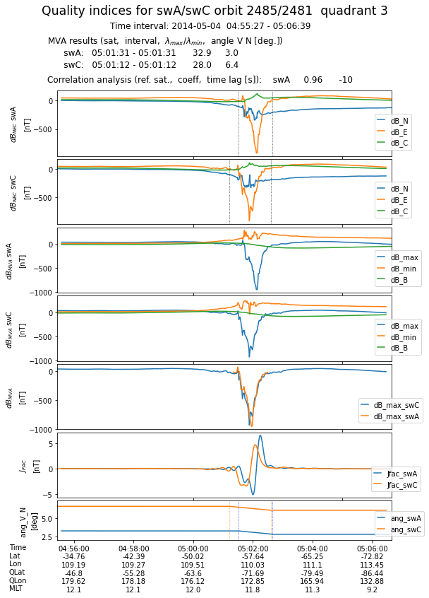
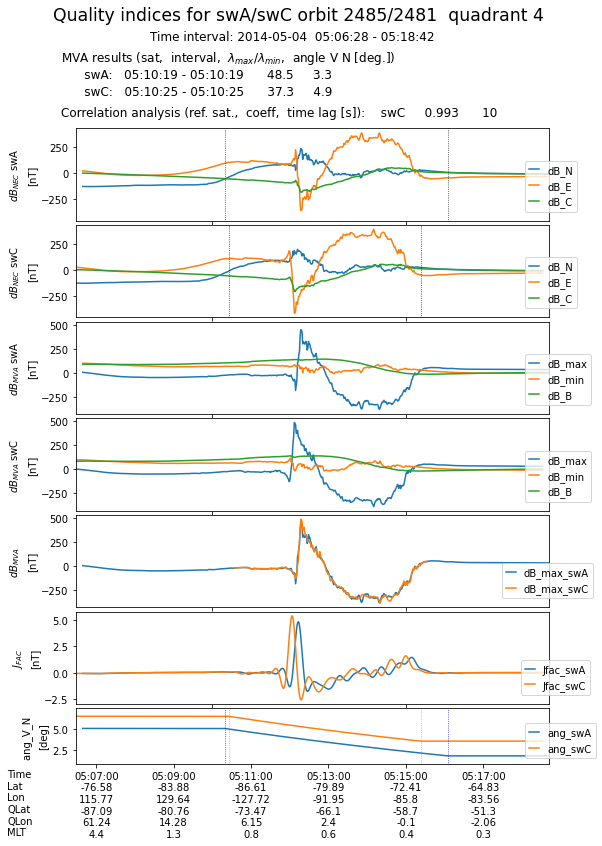
Plotting the results
Generates one plot for every 1/4 orbit. The first four panels show, for both satellites, the magnetic field perturbation in NEC and MVA frames. To illustrate the correlation between magnetic perturbations recorded by the two sensors, the fifth panel presents the evolution of maximum variance components, properly lagged in case of the reference satellite. The sixth panel shows the FAC densities obtained from filtered magnetic data, while the last panel presents the current sheet inclination wrt satellite velocity in the tangential plane.
At the end, all the plots are collected in a multi-page pdf file.
fname_plots = 'QI_sw'+sats[0]+sats[1]+'_multipage_'+str_fname + '.pdf'
list_plots = []
for jj in range(nrq):
    %run -i "plot_qi.py"
    list_plots.append(fname_fig)

list_plots_str = ' '.join(list_plots)
!gs -dNOPAUSE -sDEVICE=pdfwrite -sOUTPUTFILE={fname_plots} -dBATCH {list_plots_str}
GPL Ghostscript 9.50 (2019-10-15)
Copyright (C) 2019 Artifex Software, Inc.  All rights reserved.
This software is supplied under the GNU AGPLv3 and comes with NO WARRANTY:
see the file COPYING for details.
Processing pages 1 through 1.
Page 1
Processing pages 1 through 1.
Page 1
Processing pages 1 through 1.
Page 1
Processing pages 1 through 1.
Page 1