Minimum Variance Analysis on Swarm
Contents
Minimum Variance Analysis on Swarm
Adrian Blagau (Institute for Space Sciences, Bucharest)
Joachim Vogt (Jacobs University Bremen)
Version May 2021
This notebook accompanies the article “Multipoint Field-Aligned Current Estimates With Swarm” by A. Blagau, and J. Vogt, 2019. When used for publications, please acknowledge the authors’ work by citing the paper.
Introduction The notebook implements the algorithm of Minimum Variance Analysis (MVA) to estimate the planarity and orientation of Field Aligned Current (FAC) structures probed by the Swarm satellites. The FAC orientation can be later used to improve the FAC density estimated through the standard implementation of single-sat. method, that assumes only normal (i.e. oriented along the satellite velocity) current sheets.
The rough interval of analysis is provided by the used at the beginning; the notebook allows to inspect the data and, if needed, to refine the initial time interval. MVA is performed on the magnetic field perturbation projected on the plane perpendicular to the local average magnetic field direction. The ratio of the two eigenvalues provides an indication on the current sheet planarity while the eigenvector associated to the direction of minimum magnetic variance is associated with the current sheet orientation.
The algorithm was designed to work with low-resolution (LR) L1b data. In the LR files the missing data are marked by zero values on all magnetic field components; such points are excluded from the analysis, their value replaced by NaN, and the corresponding timetags printed on the screen.
The MVA results, provided as ASCII file, include the interval of analysis, the eigenvalues with the corresponding eigenvectors in GEOC frame, the angle of FAC inclination wrt sat. velocity measured in the tangential plane, and the components of magnetic field perturbation in the proper (i.e. current sheet) frame. The evolution of magnetic field perturbation, FAC density and inclination, as well as the hodograph of magnetic field perturbation in the plane perpendicular to the average magnetic field are plotted on screen and saved as eps file.
Importing useful libraries/ functions
The standard python libraries (numpy, pandas, matplotlib, …) are imported. Also, to easily follow the logical flow in the notebook, the functions listed below are read from the accompanying funcs_single_sat_MVA.py python script:
normvec : computes the unit-vectors of a vector time series
rotvecax : rotates a vector by an angle around another vector
sign_ang : returns the signed angle between two vectors
R_B_dB_in_GEOC : transforms in GEO Cartesian frame the satellite position (initially in spherical coordinates) and magnetic field & perturbation (initially in NEC)
singleJfac : computes the single-satellite FAC density
# Uncomment if necessary:
# %matplotlib inline
# Uncomment for interactivity:
# (required for selecting analysis interval)
# %matplotlib widget

import numpy as np
import pandas as pd
from scipy import signal
from scipy.interpolate import interp1d
import datetime as dtm
import matplotlib.pyplot as plt
import matplotlib.dates as mdt
from matplotlib.widgets import SpanSelector
from viresclient import SwarmRequest

from funcs_fac import *

import warnings
warnings.filterwarnings('ignore')
Definitions of convenience functions
Function to perform the MVA on an array of 3D vectors. To do the analysis in a plane (e.g. perpendicular to the local average magnetic field), the normal to that plane cdir (3D vector) should be specified.
def mva(v, cdir = None):
    # returns results of MVA on the array of 3D vector v. If cdir (3D vector)
    # is provided, the analysis is performed in the plane perpendiculat to it
    v_cov = np.cov(v, rowvar=False, bias=True)
    if cdir is not None:
        ccol = cdir.reshape(3,1)
        cunit = ccol / np.linalg.norm(ccol)
        d_mat = (np.identity(3) - np.dot(cunit,cunit.T))
        v_cov = np.matmul(np.matmul(d_mat, v_cov), d_mat)
    return np.linalg.eigh(v_cov)
Function to manually select the analysis interval by dragging the mouse pointer on the screen.
def onselect(xmin, xmax):
    nrl = len(ax2.lines)
    ax2.lines[nrl-1].remove()
    ax2.lines[nrl-2].remove()
    span_sel['beg'], span_sel['end'] = xmin, xmax
    ax2.axvline(xmin, ls='--', c='r')
    ax2.axvline(xmax, ls='--', c='r')
Input parameters
As input parameters, the user specifies the time-interval and the satellite. To allow for a refined analysis, the algorithm actually downloads Swarm data recorded on a larger, i.e. half-orbit time span, and offers the possibility to modify the analysis interval specified below. To compute the magnetic field perturbation, the algorithm relies on CHAOS magnetic model(s), but the user can select another model available on the VirES platform.
# Time range, satellites, and magnetic model in format '%Y-%m-%dT%H:%M:%S'

dtime_beg = '2015-03-17T08:51:54'
dtime_end = '2015-03-17T08:57:11'

sat = ['C']

use_filter = True   # 'True' for filtering the data
Bmodel = "CHAOS-all='CHAOS-Core'+'CHAOS-Static'+'CHAOS-MMA-Primary'+'CHAOS-MMA-Secondary'"
Data retrieval and preparation
Reads from VirES the sat. position (Rsph), magnetic L1b measurement (Bnec), and magnetic field model (Bmod). Auxiliary parameters QDLat, QDLon, and MLT, used when plotting the results, are retrieved as well. Time instances when the magnetic measurements assume zero values (indicative of data gaps in L1b low-resolution files) are replace by NaN. Computes the magnetic perturbation (in NEC) and, if no data gaps are present, applies a low-pass filter.
request = SwarmRequest()
# identify the right half-orbit interval
orb = request.get_orbit_number(sat[0], dtime_beg, mission='Swarm')
orb_beg, orb_end = request.get_times_for_orbits(orb, orb, mission='Swarm', spacecraft=sat[0])
half_torb = (orb_end - orb_beg)/2.
dtm_beg = dtm.datetime.fromisoformat(dtime_beg)
dtm_end = dtm.datetime.fromisoformat(dtime_end)
if dtm_beg - orb_beg < half_torb:
    large_beg, large_end = orb_beg, orb_beg + half_torb
else:
    large_beg, large_end = orb_beg + half_torb, orb_end

# download the Swarm data
request.set_collection("SW_OPER_MAG"+sat[0]+"_LR_1B")
request.set_products(measurements=["B_NEC"],
                         auxiliaries=['QDLat','QDLon','MLT'],
                         models=[Bmodel],
                         sampling_step='PT1S')
dat = request.get_between(start_time = large_beg,
                               end_time = large_end,
                               asynchronous=False)
print('Used MAG L1B file: ', dat.sources[1])
dat_df = dat.as_dataframe()

# set B_NEC data gaps (zero magnitude in L1b LR files) to NaN.
# impose no filtering if there are missing data points.
ind_gaps = np.where(\
        np.linalg.norm(np.stack(dat_df['B_NEC'].values), axis = 1)==0)[0]
if len(ind_gaps):
    dat_df, timegaps = GapsAsNaN(dat_df, ind_gaps)
    print('NR. OF MISSING DATA POINTS: ', len(ind_gaps))
    print(timegaps.values)
    print('NO FILTERING IS PERFORMED')
    use_filter = False

ti = dat_df.index

# store position, magnetic field and magnetic model vectors as data array
Rsph = dat_df[['Latitude','Longitude','Radius']].values
Bnec = np.stack(dat_df['B_NEC'].values, axis=0)
Bmod = np.stack(dat_df['B_NEC_CHAOS-all'].values, axis=0)
dBnec = Bnec - Bmod

# if possible, filter the magnetic field perturbation
if use_filter:
    fc, fs = 1./20, 1  # Cut-off and sampling frequency in s
    bf, af = signal.butter(5, fc / (fs / 2), 'low')
    dBnec_flt = signal.filtfilt(bf, af, dBnec, axis=0)
Used MAG L1B file: SW_OPER_MAGC_LR_1B_20150317T000000_20150317T235959_0505_MDR_MAG_LR
Computes the (Cartesian) position vector R, magnetic field B, and magnetic field perturbation dB in the GEOC frame. The un-filtered and, when possible, filtered current density, i.e. jb and respectively jb_flt, are computed to better assess the selection of MVA interval. Store quantities in DataFrame structures
R, B, dB = R_B_dB_in_GEOC(Rsph, Bnec, dBnec)
tt, Rmid, jb,_,_,_,_,_ = singleJfac(ti, R, B, dB)
jb_df = pd.DataFrame(jb, columns=['FAC'], index=tt)

if use_filter:
    R, B, dB_flt = R_B_dB_in_GEOC(Rsph, Bnec, dBnec_flt)
    tt, Rmid, jb_flt,_,_,_,_,_ = singleJfac(ti, R, B, dB_flt)
    jb_flt_df = pd.DataFrame(jb_flt, columns=['FAC_flt'], index=tt)

# eV2d is the satellite velocity in the tangent plane (i.e. perpendicular to position vector)
V3d = R[1:,:] - R[:-1,:]
eV3d, eRmid = normvec(V3d), normvec(Rmid)
eV2d = normvec(np.cross(eRmid, np.cross(eV3d, eRmid)))

dBnec_df = pd.DataFrame(dBnec, columns=['dB N', 'dB E', 'dB C'], index=ti)
dB_df = pd.DataFrame(dB, columns=['dB Xgeo', 'dB Ygeo', 'dB Zgeo'], index=ti)
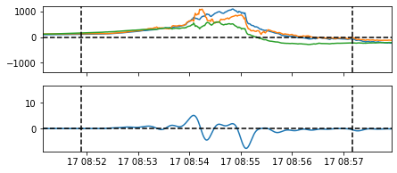
Selection of analysis interval
The initial interval of analysis is indicated on a plot that presents the magnetic field perturbation and current density (when possible, the filtered current density is preferred). If the user wants to inspect the data he/she can zoom/pan both on x and y axes after clicking the ✥ button of the interactive window (displayed at the bottom). To select another interval for MVA, click again on the ✥ button, press left mouse button and drag to select a region in the top panel.
tmarg = dtm.timedelta(seconds=45)
fig, (ax1, ax2) = plt.subplots(2, figsize=(7, 3), sharex='all')
ax1.plot(dB_df)
ax1.set_xlim(xmin = dtm_beg - tmarg, xmax = dtm_end + tmarg)
ax1.axvline(pd.to_datetime(dtime_beg), ls='--', c='k')
ax1.axvline(pd.to_datetime(dtime_end), ls='--', c='k')
ax1.axhline(0, ls='--', c='k')
if use_filter:
    ax2.plot(jb_flt_df)
else:
    ax2.plot(jb_df)
ax2.axhline(0, ls='--', c='k')
ax2.axvline(pd.to_datetime(dtime_beg), ls='--', c='k')
ax2.axvline(pd.to_datetime(dtime_end), ls='--', c='k')
span = SpanSelector(ax1, onselect, 'horizontal', useblit=True,
            span_stays=True, rectprops=dict(alpha=0.2, facecolor='red'))
Minimum Variance Analysis
Updates the analysis interval if needed and applies the MVA in the plane perpendicular to the average magnetic field direction. The current sheet normal is provided by the eigenvector associated with the minimum magnetic variance, while the sense of direction is chosen according to the sat. velocity
# update MVA interval if span has been selected
tmva_int = np.array([dtime_beg, dtime_end], dtype='datetime64')
if any([s != 0 for s in span.extents]):
    tmva_int = np.array(mdt.num2date(span.extents), dtype='datetime64')
# select quantities for MVA interval and remove NaN points
indok = np.where((ti >= tmva_int[0]) & (ti <= tmva_int[1]) & ~np.isnan(dB[:,0]))[0]
dB_int, B_int = dB[indok,:], B[indok,:]
B_ave = np.average(B_int, axis = 0)
B_unit = B_ave / np.linalg.norm(B_ave)
# apply constrained MVA
eigval,eigvec = mva(dB_int, cdir=B_unit)
# select the minvar orientation according to sat. velocity
eV3d_ave = np.average(eV3d[indok[:-1]], axis = 0)
mindir = eigvec[:,1]
if np.sum(mindir*eV3d_ave) < 0:
    mindir = -eigvec[:,1]
maxdir = np.cross(B_unit, mindir)

print('MVA interval: ', tmva_int)
print('B_unit= %10.2f'%eigval[0], np.round(B_unit, decimals=4))
print('mindir= %10.2f'%eigval[1], np.round(mindir, decimals=4))
print('maxdir= %10.2f'%eigval[2], np.round(maxdir, decimals=4))
MVA interval:  ['2015-03-17T08:51:54' '2015-03-17T08:57:11']
B_unit=       0.00 [ 0.5946 -0.196  -0.7798]
mindir=    9323.79 [-0.3277  0.8265 -0.4577]
maxdir=  250660.98 [0.7342 0.5277 0.4272]
Transforms the magnetic perturbation in the MVA (proper) frame. It also calculates the FAC inclination wrt sat. velocity in the tangential plane and corrects the FAC density estimation accordingly.
# transform magnetic perturbation in MVA frame
geo2mva = np.stack((B_unit, mindir, maxdir), axis=1)
dBmva_df= pd.DataFrame(np.matmul(dB_df.values, geo2mva),
                        columns=['dB B', 'dB min', 'dB max'], index=ti)

# compute the FAC inclination wrt sat. velocity in the tangential plane
eN2d, ang = eV2d.copy(), np.zeros(len(tt))
eN2d[indok[:-1]] = \
    normvec(np.cross(eRmid[indok[:-1]], np.cross(mindir, eRmid[indok[:-1]])))

cross_v_n = np.cross(eV2d[indok[:-1]], eN2d[indok[:-1]])
sign_ang = np.sign(np.sum(eRmid[indok[:-1]]*cross_v_n, axis=-1))
ang[indok[:-1]]  = \
        np.degrees(np.arcsin(sign_ang*np.linalg.norm(cross_v_n, axis=-1)))
ang[0:indok[0]] = ang[indok[0]]
ang[indok[-1]:] = ang[indok[-2]]

# DataFrames with FAC inclination and density corrected for inclination
ang_df = pd.DataFrame(ang, columns=['ang_v_n'], index=tt)
tt, Bmid, jb_inc, _, _, _, _, _ = singleJfac(ti, R, B, dB, alpha=ang)
jb_inc_df = pd.DataFrame(jb_inc, columns=['FAC_inc'], index=tt)
if use_filter:
    tt, Bmid, jb_inc_flt, _, _, _, _, _ = singleJfac(ti, R, B, dB_flt, alpha=ang)
    jb_inc_flt_df = pd.DataFrame(jb_inc_flt, columns=['FAC_inc_flt'], index=tt)
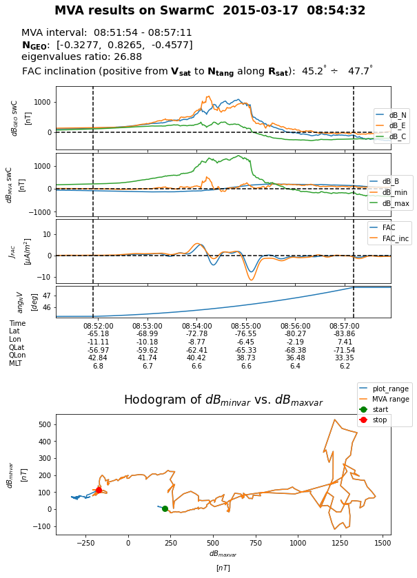
Plotting and saving the MVA results
The plot presents (i) the magnetic field perturbation in NEC, (ii) magnetic field perturbation in the proper frame, (iii) a comparison between the standard and corrected for inclination FAC density estimates (filtered quantities are preferred), and (iv) the angle (in degree) of FAC inclination in the tangential plane wrt satellite velocity vector. The hodograph of magnetic field perturbation in the plane perpendicular to the average magnetic field is presented as well. The ASCII file contains the MVA results and the magnetic field perturbation in the proper (MVA associated) frame.
%run -i "plot_and_save_single_sat_MVA.py"