Dual-sat FAC density estimation with Swarm
Contents
Dual-sat FAC density estimation with Swarm
Adrian Blagau (Institute for Space Sciences, Bucharest)
Joachim Vogt (Jacobs University Bremen)
Version June 2021
This notebook accompanies the article “Multipoint Field-Aligned Current Estimates With Swarm” by A. Blagau, and J. Vogt, 2019. When used for publications, please acknowledge the authors’ work by citing the paper.
Introduction The notebook makes use of the dual-s/c gradient estimation method, developed in Vogt et al., 2013, to estimates the field-aligned current (FAC) density based on the lower satellite (Swarm A and C) data or, when Swarm forms a close configuration, by combining data from the upper satellite (Swarm B) and one of the lower satellites.
Four point planar configurations (quads) are formed by combining virtual satellite positions, separated along the orbit, and the the Ampère’s law, in the least-square (LS) formulation, is used to infer the current flowing through the quad. Then, the FAC density is estimated by considering the orientation of local magnetic field wrt quad normal. The LS approach has several advantages over the ESA L2 algorithm since it provides stabler solutions, can be applied on a more general spacecraft configuration, and offers a robust error estimation scheme. Consequently, the method provides significantly more data near the singularity where the satellites’ orbits intersect, allows FAC estimation with configurations that involves the upper Swarm satellite, or to fine tune the constellation geometry to the problem at hand. A detailed discussion on applying the LS dual-s/c method in the context of Swarm is provided in Blagau and Vogt, 2019.
In the Input parameters section, the user specifies the interval and the satellites used in the analysis, as well as the parameters that specify the quad configuration, i,e, the along track separation and the time shift needed to align the sensors. When the lower satellites are used, the later can actually be calculated from the orbital elements.
Importing useful libraries (numpy, pandas, matplotlib, …)
# Uncomment if necessary:
# %matplotlib inline
# Uncomment for interactivity:
# %matplotlib widget

import numpy as np
import pandas as pd
from scipy import signal
import matplotlib.pyplot as plt
import datetime as dtm
import matplotlib.dates as mdt

import warnings
warnings.filterwarnings('ignore')
Preparing to access ESA’s Swarm mission data and models from VirES environment
from viresclient import SwarmRequest
request = SwarmRequest()
Defining some convenience functions
Computing the parameters of a low-pass Butterworth filter, if one decides to filter the data
fs = 1  # Sampling frequency
fc = 1./20.  # Cut-off frequency of a 20 s low-pass filter
w = fc / (fs / 2)  # Normalize the frequency
butter_ord = 5
bf, af = signal.butter(butter_ord, w, 'low')
Defining the recivec2s function, to compute the reciprocal vectors of a 4 point planar configuration. See Vogt et al., 2013 for details.
def recivec2s(R4s):
    # work in the mesocenter frame
    Rmeso = np.mean(R4s, axis=-2)
    R4smc = R4s - Rmeso[:, np.newaxis, :]
    Rtens = np.sum(np.matmul(R4smc[:,:,:,None],R4smc[:,:,None, :]), axis = -3)
    eigval, eigvec = np.linalg.eigh(Rtens)
    # avoid eigenvectors flipping direction
    # for that, impose N to be closer to radial direction
    nprov = np.squeeze(eigvec[:,:,0])    # provisional normal
    cosRN = np.squeeze(np.matmul(Rmeso[...,None,:],nprov[...,:,None]))
    iposr = cosRN < 0
    eigvec[iposr,:,:] = -eigvec[iposr,:,:]
    # minimum variance direction is along normal N
    nuvec = np.squeeze(eigvec[:,:,0])
    intvec = np.squeeze(eigvec[:,:,1])
    maxvec = np.squeeze(eigvec[:,:,2])
    # nonplanarity and condition number
    nonplan = eigval[:,0]/eigval[:,2]
    condnum = eigval[:,2]/eigval[:,1]
    qtens = 1./eigval[:,2,np.newaxis,np.newaxis]*np.matmul(maxvec[:,:,None],maxvec[:,None, :]) +\
        1./eigval[:,1,np.newaxis,np.newaxis]*np.matmul(intvec[:,:,None],intvec[:,None, :])
    # Q4s are the planar canonical base vectors
    Q4s = np.squeeze(np.matmul(qtens[:,None, :,:],R4smc[:,:,:,None]))
    # trace of the position and reciprocal tensor
    tracer = np.sum(np.square(np.linalg.norm(R4smc, axis = -1)), axis=-1)
    traceq = np.sum(np.square(np.linalg.norm(Q4s, axis = -1)), axis=-1)

    return Q4s, Rmeso, nuvec, condnum, nonplan, tracer, traceq
Input parameters
Specifying the time interval and the pair of satellites used in the analysis. To construct the quad configuration, one have to specify the time shift (tshift) needed to align the sensors, and the along-track separation (dt_along) between the quad’s corners. The time-shift can be explicitly set here or, when tshift is not defined, it’s optimal value is calculated from the orbital elements (works mainly for configurations based on the lower satellites).
dtime_beg = '2014-05-04T16:04:00'
dtime_end = '2014-05-04T16:11:00'

sats = ['A','C']

dt_along = 5        # along track separation
# tshift = [0, 13]   # optional time-shift between sensors.
                    # When not defined, it is estimated below

# sats = ['B','C']
# tshift = [0, 3]
# sats = ['B','A']
# tshift = [0, 13]
To reduce the influence of local magnetic fluctuations, filtered data should be used. Bmodel designates the magnetic model used to calculate magnetic field perturbations. db represents the amplitude, in nT, of effective magnetic noise (instrumental error). angTHR is the threshold minimum value needed to recover the FAC density from the radial current density and errTHR is the accepted error level for the FAC density.
use_filter = True   # 'True' (for filtering the data) or 'False'
Bmodel="CHAOS-all='CHAOS-Core'+'CHAOS-Static'+'CHAOS-MMA-Primary'+'CHAOS-MMA-Secondary'"
db = 0.2 if use_filter else 0.5
angTHR = 30.
errTHR = 0.1
Data retrieval
Reading from VirES the sat. position (Rsph), magnetic L1b low resolution data (Bsw), and magnetic field model (Bmod). The auxiliary data, i.e. quasi-dipole latitude and longitude, magnetic local time, and longitude of the ascending node, are also retrieved.
dti = pd.date_range(start = pd.Timestamp(dtime_beg).ceil('s'),\
                    end = pd.Timestamp(dtime_end).floor('s'), freq='s')
ndti = len(dti)
nsc = len(sats)
datagaps={}
Rsph, Bsw, Bmod = (np.full((ndti,nsc,3),np.nan) for i in range(3))
Aux = np.full((ndti,nsc,4),np.nan)

for sc in range(nsc):
    request.set_collection("SW_OPER_MAG"+sats[sc]+"_LR_1B")
    request.set_products(measurements=["B_NEC"],
                         auxiliaries=['QDLat','QDLon','MLT','AscendingNodeLongitude'],
                         models=[Bmodel],
                         sampling_step="PT1S")
    data = request.get_between(start_time = dti[0].to_pydatetime(), \
                end_time = dti[-1].to_pydatetime()+dtm.timedelta(seconds=0.1), \
                asynchronous=False)
    print('Used MAG L1B file: ', data.sources[2])
    dat = data.as_dataframe()
    # interpolate at dti moments if B_NEC has data gaps, marked as zero
    # magnitude in L1b LR files. Stores position, magnetic field and
    # magnetic model vectors in corresponding data matrices
    ind_nogaps = np.where(\
        np.linalg.norm(np.stack(dat['B_NEC'].values), axis = 1)>0)[0]
    if len(ind_nogaps) != ndti:
        print('NR. OF MISSING DATA POINTS: ', ndti - len(ind_nogaps))
        for jj in range(3):
            Rsph[:,sc,jj] = np.interp(dti,dat.index[ind_nogaps],\
                                dat[['Latitude','Longitude','Radius']].values[ind_nogaps,jj])
            Bmod[:,sc,jj] = np.interp(dti,dat.index[ind_nogaps],\
                                np.stack(dat['B_NEC_CHAOS-all'].values, axis=0)[ind_nogaps,jj])
            Aux[:,sc,jj] = np.interp(dti,dat.index[ind_nogaps],\
                                dat[['QDLat','QDLon','MLT']].values[ind_nogaps,jj])
            Bsw[:,sc,jj] = np.interp(dti,dat.index[ind_nogaps],\
                                np.stack(dat['B_NEC'].values, axis=0)[ind_nogaps,jj])
        Aux[:,sc, 3] = np.interp(dti,dat.index[ind_nogaps],\
                                dat[['AscendingNodeLongitude']].values[ind_nogaps,jj])
    else:
        Rsph[:,sc,:] = dat[['Latitude','Longitude','Radius']].values
        Bmod[:,sc,:] = np.stack(dat['B_NEC_CHAOS-all'].values, axis=0)
        Aux[:,sc,:] = dat[['QDLat','QDLon','MLT','AscendingNodeLongitude']].values
        Bsw[:,sc,:] = np.stack(dat['B_NEC'].values, axis=0)

# stores data in DataFrames
colRsph = pd.MultiIndex.from_product([['Rsph'],sats,['Lat','Lon','Radius']],
                                   names=['Var','Sat','Com'])
dfRsph = pd.DataFrame(Rsph.reshape(-1,nsc*3),columns=colRsph,index=dti)

colBswBmod = pd.MultiIndex.from_product([['Bsw','Bmod'],sats,['N','E','C']],
                                   names=['Var','Sat','Com'])
dfBswBmod = pd.DataFrame(np.concatenate((Bsw.reshape(-1,nsc*3),
                                         Bmod.reshape(-1,nsc*3)),axis=1),
                         columns=colBswBmod,index=dti)

RsphBswBmod = pd.merge(dfRsph, dfBswBmod, left_index=True, right_index=True)
Used MAG L1B file: SW_OPER_MAGA_LR_1B_20140504T000000_20140504T235959_0505_MDR_MAG_LR
Used MAG L1B file: SW_OPER_MAGC_LR_1B_20140504T000000_20140504T235959_0505_MDR_MAG_LR
Preparation and data alignment
When tshift parameter is not defined, computes its optimal value. To that end, one founds the time difference in satellites’ ascending nodes and subsequently correct this value by taking into account the orbit inclination (i.e. 87.35 deg. for Swarm lower pair). This calculations works pretty accurate for configurations based on the lower satellites.
try: tshift
except NameError:
    AscNodeSats = []
    for ii in range(2):
        orb = request.get_orbit_number(sats[ii], dtime_beg, mission='Swarm')
        AscNodeSats.append(request.get_times_for_orbits(orb, orb, spacecraft=sats[ii]))
    AscLag = 0.5*(AscNodeSats[1][0] - AscNodeSats[0][0]).total_seconds() +\
              0.5*(AscNodeSats[1][1] - AscNodeSats[0][1]).total_seconds()
    print('Asc. Node time diff.: Sat',sats[0],' lags behind Sat',sats[1],'by ',AscLag,' sec.')
    # Compensate for the orbit inclination
    Rorb = np.mean(Rsph[:,0,2],axis=0)
    Torb = (AscNodeSats[0][1] - AscNodeSats[0][0]).total_seconds()
    Vorb = 2*np.pi*Rorb/Torb
    Oinc = np.deg2rad(90 - 87.35)
    dlon = np.abs((Aux[0,1,3] - Aux[0,0,3] + 180) % 360 - 180)
    Deq = dlon*2*np.pi*Rorb/360
    Tcorr = Deq*np.tan(Oinc)/Vorb
    print('Time diff. due to orbit incl. :',np.round(Tcorr,4) ,' sec.')
    tshift = [int(-np.sign(AscLag)*round(np.abs(AscLag) + Tcorr)), 0]

print('satellites: ', sats)
print('Time shift: ', tshift)
Asc. Node time diff.: Sat A  lags behind Sat C by  -8.843705  sec.
Time diff. due to orbit incl. : 1.0417  sec.
satellites:  ['A', 'C']
Time shift:  [10, 0]
Making time shift relative to the smalest element
indmin = tshift.index(min(tshift))
indmax = tshift.index(max(tshift))
tshift[indmax] = tshift[indmax] - min(tshift)
tshift[indmin] = 0
dtshift = tshift[indmax]
print('indmin, indmax = ', indmin, indmax)
print('tshift, dtshift = ', tshift, dtshift)
indmin, indmax =  1 0
tshift, dtshift =  [10, 0] 10
Introducing time shift between sensors. Keep only relevant data. To keep compatibility with the ESA FAC L2 product, the associated time stamps are those from the sensor shifted ahead, i.e. Swarm A.
ndt = ndti-dtshift
dt = dti[dtshift:]
for sc in range(nsc):
    Rsph[0:ndt,sc,:] = Rsph[tshift[sc]:ndt + tshift[sc] ,sc,:]
    Bmod[0:ndt,sc,:] = Bmod[tshift[sc]:ndt + tshift[sc] ,sc,:]
    Aux[0:ndt,sc,:] = Aux[tshift[sc]:ndt + tshift[sc] ,sc,:]
    Bsw[0:ndt,sc,:] = Bsw[tshift[sc]:ndt + tshift[sc] ,sc,:]

Rsph = np.delete(Rsph, np.s_[ndt:],0)
Bmod = np.delete(Bmod, np.s_[ndt:],0)
Aux = np.delete(Aux, np.s_[ndt:],0)
Bsw = np.delete(Bsw, np.s_[ndt:],0)
Constructing the 4-point planar configuration
Computing sats positions (R), magnetic measurements (B), and magnetic field perturbations (dB) in the global geographic (cartesian) frame. Filters the magnetic field perturbations if requested so.
R, B, dB = (np.full((ndt,nsc,3),np.nan) for i in range(3))
for sc in range(nsc):
    latsc = np.deg2rad(Rsph[:,sc,0])
    lonsc = np.deg2rad(Rsph[:,sc,1])
    radsc = 0.001*Rsph[:,sc,2]
    # prepare conversion to global cartesian frame
    clt,slt = np.cos(latsc.flat),np.sin(latsc.flat)
    cln,sln = np.cos(lonsc.flat),np.sin(lonsc.flat)
    north = np.stack((-slt*cln,-slt*sln,clt),axis=-1)
    east = np.stack((-sln,cln,np.zeros(cln.shape)),axis=-1)
    center = np.stack((-clt*cln,-clt*sln,-slt),axis=-1)
    # store cartesian position vectors in position data matrix R
    R[:,sc,:] = -radsc[...,None]*center
    # store magnetic field measurements in the same frame
    bnecsc = Bsw[:,sc,:]
    B[:,sc,:] = np.matmul(np.stack((north,east,center),axis=-1),
                              bnecsc[...,None]).reshape(bnecsc.shape)
    # store magnetic field perturbation in the same frame
    dbnecsc = Bsw[:,sc,:] - Bmod[:,sc,:]
    dB[:,sc,:] = np.matmul(np.stack((north,east,center),axis=-1),
                              dbnecsc[...,None]).reshape(dbnecsc.shape)
    if use_filter:
        dB[:,sc,:] = signal.filtfilt(bf, af, dB[:,sc,:], axis=0)
# collect all data in a single DataFrame
colRBdB = pd.MultiIndex.from_product([['R','B','dB'],sats,['x','y','z']],
                                   names=['Var','Sat','Com'])
RBdB = pd.DataFrame(np.concatenate((R.reshape(-1,nsc*3),B.reshape(-1,nsc*3),dB.reshape(-1,nsc*3)),axis=1),
                      columns=colRBdB,index=dt)
Constructing the four point configuration, with the corresponding values for R, B, and dB at each corner. Going along the quad, the points are named 0, 2, 3, 1, with 0 and 2 from the first sensor (i.e. sats[0]) and 1 and 3 from the second sensor (i.e. sats[1])
ndt4 = ndt-dt_along
R4s = np.full((ndt4,4,3),np.nan)
B4s = np.full((ndt4,4,3),np.nan)
dB4s = np.full((ndt4,4,3),np.nan)

R4s[:,0:2, :] = R[:ndt4, :, :]
R4s[:,2:, :] = R[dt_along:, :, :]
B4s[:,0:2, :] = B[:ndt4, :, :]
B4s[:,2:, :] = B[dt_along:, :, :]
dB4s[:,0:2, :] = dB[:ndt4, :, :]
dB4s[:,2:, :] = dB[dt_along:, :, :]
Computing the FAC density and other parameters
Using recivec2s() function to compute the planar canonical base vectors (Q4s), the position at mesocenter (Rmeso), the quad normal (nuvec), the condition number (condnum), nonplanarity (nonplan) and trace of the position (tracer) and reciprocal (traceq) tensors.
Q4s, Rmeso, nuvec, condnum, nonplan, tracer, traceq = recivec2s(R4s)
Estimating the curl of magnetic field perturbation curlB. Associates its normal component curlBn with an electric current of density Jfac, flowing along the magnetic field line.
Computes the direction of (un-subtracted) local magnetic field Bunit and the orientation of spacecraft plane with respect to Bunit (cosBN and angBN).\
The current density along the radial (outward) direction Jrad is also computed. Its sign depends on the hemisphere.
dt4 = dt[:ndt4].shift(1000.*(dt_along/2),freq='ms')
muo = 4*np.pi*1e-7
CurlB = np.sum( np.cross(Q4s,dB4s,axis=-1), axis=-2 )
CurlBn = np.squeeze(np.matmul(CurlB[...,None,:],nuvec[...,:,None]))
Bunit = B4s.mean(axis=-2)/np.linalg.norm(B4s.mean(axis=-2),axis=-1)[...,None]
cosBN = np.squeeze(np.matmul(Bunit[...,None,:],nuvec[...,:,None]))
angBN = np.arccos(cosBN)*180./np.pi
# FAC density
Jfac= (1e-6/muo)*pd.Series(CurlBn/cosBN,index=dt4)
# Current density along the radial (outward) direction. This depends on the hemispheres
Jrad= (1e-6/muo)*pd.Series(CurlBn,index=dt4)
The error errJ in FAC density due to (mutually uncorrelated and isotropic) instrumental noise δB is evaluated by considering a flat value of db nT.
Find (and exclude) data points / intervals when the value of the current density is not reliable estimated:
- when the quad becomes too stretched (close to the lopes) and errJ increases, defined as errJ grater than a threshold value set in errTHR. This affects both Jfac and Jrad
- when the B vector is too close to the spacecraft plane, i.e. below a threshold value set in angTHR. This situation affects only Jfac and is not encounter when the lower satellites pair is used.
def group_consecutive(data, stepsize=1):
    return np.split(data, np.where(np.diff(data) != stepsize)[0]+1)
errJ = 1e-6*db/muo*pd.Series(np.sqrt(traceq)/np.absolute(cosBN),index=dt4)
texcl = errJ.values > errTHR
tang = (np.absolute(angBN) < 90 + angTHR) & (np.absolute(angBN) > 90 - angTHR)
Jfac.values[texcl] = np.nan
Jrad.values[texcl] = np.nan
Jfac.values[tang] = np.nan

# Computes the limits of the exclusion zone (if present)
EZstart, EZstop = ([] for i in range(2))
EZind = np.where(texcl)[0]
if len(EZind):
    grpEZind = group_consecutive(EZind)
    for ii in range(len(grpEZind)):
        EZstart.append(dt4[grpEZind[ii][0]] if grpEZind[ii][0] >= 0 else [])
        EZstop.append(dt4[grpEZind[ii][-1]] if grpEZind[ii][-1] < ndt4 else [])

# Computes the limits of the small angle zone (if present)
ANGstart, ANGstop = ([] for i in range(2))
ANGind = np.where(tang)[0]
if len(ANGind):
    grpANGind = group_consecutive(ANGind)
    for ii in range(len(grpANGind)):
        ANGstart.append(dt4[grpANGind[ii][0]] if grpANGind[ii][0] >= 0 else [])
        ANGstop.append(dt4[grpANGind[ii][-1]] if grpANGind[ii][-1] < ndt4 else [])
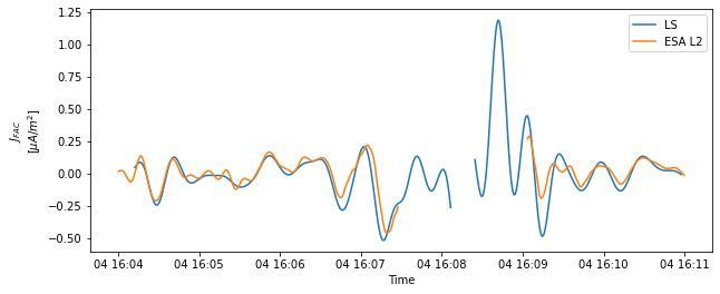
Reading two-sat. FAC estimate from the ESA L2 product for a quick comparison.
request.set_collection('SW_OPER_FAC_TMS_2F')
request.set_products(measurements=["FAC"], sampling_step="PT1S")
data = request.get_between(start_time = dtime_beg,
                               end_time = dtime_end,
                               asynchronous=False)
print('Used FAC file: ', data.sources[0])
FAC_L2 = data.as_dataframe()

plt.figure(figsize = [10,4])
plt.plot(Jfac, label = 'LS')
plt.plot(FAC_L2['FAC'], label = 'ESA L2')
plt.ylabel('$J_{FAC}$\n[$\mu A/m^2$]')
plt.xlabel('Time')
plt.legend()
Used FAC file: SW_OPER_FAC_TMS_2F_20140504T000000_20140504T235959_0301
<matplotlib.legend.Legend at 0x7ff41c513640>
Plotting and saving the results
The script below produces a plot, to be saved locally together with an ASCII file.
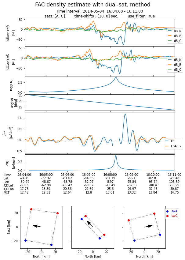
The generated plot presents:
the NEC components of the magnetic field perturbation, dB, for the two satellites. A common range along y axes is used
the logarithm of the condition number, CN
angle between the normal to the spacecraft plane and the direction of local ambient magnetic field.
comparison between the FAC density estimated with the LS method and the ESA L2 FAC product obtained from the dual-s/c method.
the FAC estimation errors due to instrumental noise
The values for tick labels refer to the trailing position of the sensor shifted ahead.
On the bottom, the 4-point configuration is shown at three instances (i.e. beginning, middle, and end of the interval) projected on the NE plane of the local NEC coordinate frame tied to the mesocenter. The velocity vector of the mesocenter is also indicated.
%run -i "plot_and_save_dual_sat.py"